pacman::p_load(sf, tidyverse)Hands-on Exercise 1a: Geospatial Data Wrangling with R
1 Geospatial Data Science with R
1.1 Learning Outcomes
Geospatial Data Science is the process of importing, wrangling, integrating, and processing geographically referenced data sets. In this hands-on exercise, the goal is to learn how to perform geospatial data science tasks in R by using sf package.
By the end of this hands-on exercise the following competencies should be acquired:
- installing and loading sf and tidyverse packages into R environment,
- importing geospatial data by using appropriate functions of sf package,
- importing aspatial data by using appropriate function of readr package,
- exploring the contents of simple feature data frame by using appropriate Base R and sf functions,
- assigning or transforming coordinate systems by using using appropriate sf functions,
- converting an aspatial data into a sf data frame by using appropriate function of sf package,
- performing geoprocessing tasks by using appropriate functions of sf package,
- performing data wrangling tasks by using appropriate functions of dplyr package and
- performing Exploratory Data Analysis (EDA) by using appropriate functions from ggplot2 package.
Note: It is encouraged to read the reference guide of each function, especially the input data requirements, syntext and argument option before using them.
1.2 Data Acquisition
Data is key to data analytics which also includes geospatial analytics. Hence, before analysis it is required to assemble the necessary data. For this hands-on exercise the data will be extracted from the following sources:
- Master Plan 2014 Subzone Boundary (Web) from data.gov.sg
- Pre-Schools Location from data.gov.sg
- Cycling Path from LTADataMall
- Latest version of Singapore Airbnb listing data from Inside Airbnb
Note: This section does not merely constitute to extracting the necessary data sets. It also aims to introduce the usage of publicly available data sets.
1.2.1 Extracting the geospatial data sets
The following steps have been carried out for extraction of the data sets:
In the Hands-on_Ex01 folder, a sub-folder called data is created. Then, inside the data sub-folder, two other sub-folders are created and are named geospatial and aspatial respectively.
The downloaded zipped files Master Plan 2014 Subzone Boundary (Web), Pre-Schools Location and Cycling Path are placed into geospatial sub-folder and unzipped. The unzipped files are then copied from their respective sub-folders and placed inside the geospatial sub-folder.
1.2.2 Extracting the aspatial data set
The downloaded listing data file is extracted. And placed in the Downloads folder by cutting and pasting the listing.csv file into the aspatial sub-folder.
1.3 Getting Started
THe following 2 R packages will be used for this hands-on exercise:
- sf for importing, managing, and processing geospatial data, and
- tidyverse for performing data science tasks such as importing, wrangling and visualising data.
Tidyverse consists of a family of R packages. In this hands-on exercise, the following packages will be used:
- readr for importing csv data,
- readxl for importing Excel worksheet,
- tidyr for manipulating data,
- dplyr for transforming data, and
- ggplot2 for visualising data
Note
The code chunk below uses p_load() of pacman package to check if sf and tidyverse packages are installed in the computer. If they are, then they will be launched into R.
1.4 Importing Geospatial Data
In this section, the geospatial data is imported into R by using st_read() of sf package:
MP14_SUBZONE_WEB_PL, a polygon feature layer in ESRI shapefile format,CyclingPath, a line feature layer in ESRI shapefile format, andPreSchool, a point feature layer in kml file format.
1.4.1 Importing polygon feature data in shapefile format
The code chunk below uses st_read() function of sf package to import MP14_SUBZONE_WEB_PL shapefile into R as a polygon feature data frame. Note that when the input geospatial data is in shapefile format, two arguments will be used, namely: dsn to define the data path and layer to provide the shapefile name.
Also note that no extension such as .shp, .dbf, .prj and .shx are needed.
mpsz = st_read(dsn = "data/geospatial",
                  layer = "MP14_SUBZONE_WEB_PL")
Reading layer `MP14_SUBZONE_WEB_PL' from data source
`C:\zjho008\ISSS626-GAA\Hands-on_Ex\Hands-on_Ex01\data\geospatial'
using driver `ESRI Shapefile'
Simple feature collection with 323 features and 15 fields
Geometry type: MULTIPOLYGON
Dimension: XY
Bounding box: xmin: 2667.538 ymin: 15748.72 xmax: 56396.44 ymax: 50256.33
Projected CRS: SVY21The message above reveals that the geospatial objects are multipolygon features. There are a total of 323 multipolygon features and 15 fields in mpsz simple feature data frame. mpsz is in svy21 projected coordinates systems. The bounding box provides the x extend and y extend of the data.
1.4.2 Importing polyline feature data in shapefile form
Again, the code chunk below uses st_read() function of sf package to import CyclingPath shapefile into R but as a line feature data frame.
cyclingpath = st_read(dsn = "data/geospatial",
                         layer = "CyclingPathGazette")
Reading layer `CyclingPathGazette' from data source
`C:\zjho008\ISSS626-GAA\Hands-on_Ex\Hands-on_Ex01\data\geospatial'
using driver `ESRI Shapefile'
Simple feature collection with 3138 features and 2 fields
Geometry type: MULTILINESTRING
Dimension: XY
Bounding box: xmin: 11854.32 ymin: 28347.98 xmax: 42644.17 ymax: 48948.15
Projected CRS: SVY21The message above reveals that the geospatial objects are linestring features. There are a total of 3138 features and 2 fields in cyclingpath linestring feature data frame and it is in svy21 projected coordinates system as well.
1.4.3 Importing GIS data in kml format
The PreSchoolsLocation is in kml format. The code chunk below will be used to import the kml file into R. Notice that in the code chunk below, the complete path and the kml file extension were provided.
preschool = st_read("data/geospatial/PreSchoolsLocation.kml")Reading layer `PRESCHOOLS_LOCATION' from data source
`C:\zjho008\ISSS626-GAA\Hands-on_Ex\Hands-on_Ex01\data\geospatial\PreSchoolsLocation.kml'
using driver `KML'
Simple feature collection with 2290 features and 2 fields
Geometry type: POINT
Dimension: XYZ
Bounding box: xmin: 103.6878 ymin: 1.247759 xmax: 103.9897 ymax: 1.462134
z_range: zmin: 0 zmax: 0
Geodetic CRS: WGS 84The message above reveals that preschool is a point feature data frame. There are a total of 2290 features and 2 fields. It is different from the previous two simple feature data frames, preschool is in wgs84 coordinates system.
1.5 Checking the Content of A Simple Feature Data Frame
In this sub-section, it illustrates different ways to retrieve information related to the content of a simple feature data frame.
1.5.1 Working with st_geometry()
The column in the sf data.frame that contains the geometries is a list, of class sfc. The geometry list-column can be retrieved in this case by mpsz$geom or mpsz[[1]], but more a generic way uses st_geometry() as shown in the code chunk below.
st_geometry(mpsz)Geometry set for 323 features
Geometry type: MULTIPOLYGON
Dimension: XY
Bounding box: xmin: 2667.538 ymin: 15748.72 xmax: 56396.44 ymax: 50256.33
Projected CRS: SVY21
First 5 geometries:Note: Note that the print only displays basic information of the feature class such as type of geometry, the geographic extent of the features and the coordinate system of the data.
1.5.2 Working with glimpse()
Besides the basic feature information, more can be learnt about the associated attribute information in the data frame. This where glimpse() of dplyr is handy as shown in the code chunk below.
glimpse(mpsz)Rows: 323
Columns: 16
$ OBJECTID <int> 1, 2, 3, 4, 5, 6, 7, 8, 9, 10, 11, 12, 13, 14, 15, 16, 17, …
$ SUBZONE_NO <int> 1, 1, 3, 8, 3, 7, 9, 2, 13, 7, 12, 6, 1, 5, 1, 1, 3, 2, 2, …
$ SUBZONE_N <chr> "MARINA SOUTH", "PEARL'S HILL", "BOAT QUAY", "HENDERSON HIL…
$ SUBZONE_C <chr> "MSSZ01", "OTSZ01", "SRSZ03", "BMSZ08", "BMSZ03", "BMSZ07",…
$ CA_IND <chr> "Y", "Y", "Y", "N", "N", "N", "N", "Y", "N", "N", "N", "N",…
$ PLN_AREA_N <chr> "MARINA SOUTH", "OUTRAM", "SINGAPORE RIVER", "BUKIT MERAH",…
$ PLN_AREA_C <chr> "MS", "OT", "SR", "BM", "BM", "BM", "BM", "SR", "QT", "QT",…
$ REGION_N <chr> "CENTRAL REGION", "CENTRAL REGION", "CENTRAL REGION", "CENT…
$ REGION_C <chr> "CR", "CR", "CR", "CR", "CR", "CR", "CR", "CR", "CR", "CR",…
$ INC_CRC <chr> "5ED7EB253F99252E", "8C7149B9EB32EEFC", "C35FEFF02B13E0E5",…
$ FMEL_UPD_D <date> 2014-12-05, 2014-12-05, 2014-12-05, 2014-12-05, 2014-12-05…
$ X_ADDR <dbl> 31595.84, 28679.06, 29654.96, 26782.83, 26201.96, 25358.82,…
$ Y_ADDR <dbl> 29220.19, 29782.05, 29974.66, 29933.77, 30005.70, 29991.38,…
$ SHAPE_Leng <dbl> 5267.381, 3506.107, 1740.926, 3313.625, 2825.594, 4428.913,…
$ SHAPE_Area <dbl> 1630379.27, 559816.25, 160807.50, 595428.89, 387429.44, 103…
$ geometry <MULTIPOLYGON [m]> MULTIPOLYGON (((31495.56 30..., MULTIPOLYGON (…The glimpse() report reveals the data type of each fields. For example FMEL-UPD_D field is in date data type and X_ADDR, Y_ADDR, SHAPE_Length and SHAPE_Area fields are all in double-precision values.
1.5.3 Working with head()
At times, to reveal the complete information of a feature object, head() of Base R can be used.
head(mpsz, n=5)Simple feature collection with 5 features and 15 fields
Geometry type: MULTIPOLYGON
Dimension: XY
Bounding box: xmin: 25867.68 ymin: 28369.47 xmax: 32362.39 ymax: 30435.54
Projected CRS: SVY21
OBJECTID SUBZONE_NO SUBZONE_N SUBZONE_C CA_IND PLN_AREA_N
1 1 1 MARINA SOUTH MSSZ01 Y MARINA SOUTH
2 2 1 PEARL'S HILL OTSZ01 Y OUTRAM
3 3 3 BOAT QUAY SRSZ03 Y SINGAPORE RIVER
4 4 8 HENDERSON HILL BMSZ08 N BUKIT MERAH
5 5 3 REDHILL BMSZ03 N BUKIT MERAH
PLN_AREA_C REGION_N REGION_C INC_CRC FMEL_UPD_D X_ADDR
1 MS CENTRAL REGION CR 5ED7EB253F99252E 2014-12-05 31595.84
2 OT CENTRAL REGION CR 8C7149B9EB32EEFC 2014-12-05 28679.06
3 SR CENTRAL REGION CR C35FEFF02B13E0E5 2014-12-05 29654.96
4 BM CENTRAL REGION CR 3775D82C5DDBEFBD 2014-12-05 26782.83
5 BM CENTRAL REGION CR 85D9ABEF0A40678F 2014-12-05 26201.96
Y_ADDR SHAPE_Leng SHAPE_Area geometry
1 29220.19 5267.381 1630379.3 MULTIPOLYGON (((31495.56 30...
2 29782.05 3506.107 559816.2 MULTIPOLYGON (((29092.28 30...
3 29974.66 1740.926 160807.5 MULTIPOLYGON (((29932.33 29...
4 29933.77 3313.625 595428.9 MULTIPOLYGON (((27131.28 30...
5 30005.70 2825.594 387429.4 MULTIPOLYGON (((26451.03 30...Note: A useful argument of head() is that it allows the user to select the number of records to display (i.e. the n argument).
1.6 Plotting the Geospatial Data
In geospatial data science, only ooking at the feature information is not enough. We are also interested in visualising the geospatial features. This is when plot() of R Graphic comes in very handy as shown in the code chunk below.
plot(mpsz)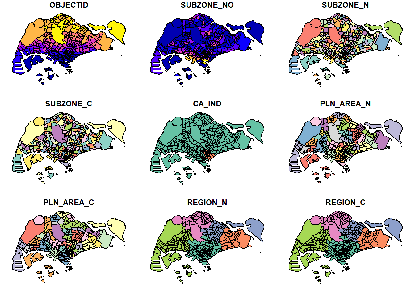
The default plot of an sf object is a multi-plot of all attributes, up to a reasonable maximum as shown above. However, the geometry can only be chosen for plotting by using the code chunk below.
plot(st_geometry(mpsz))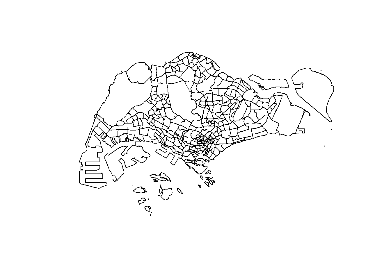
Alternatively, the plot of the sf object can also be chosen by using a specific attribute as shown in the code chunk below.
plot(mpsz["PLN_AREA_N"])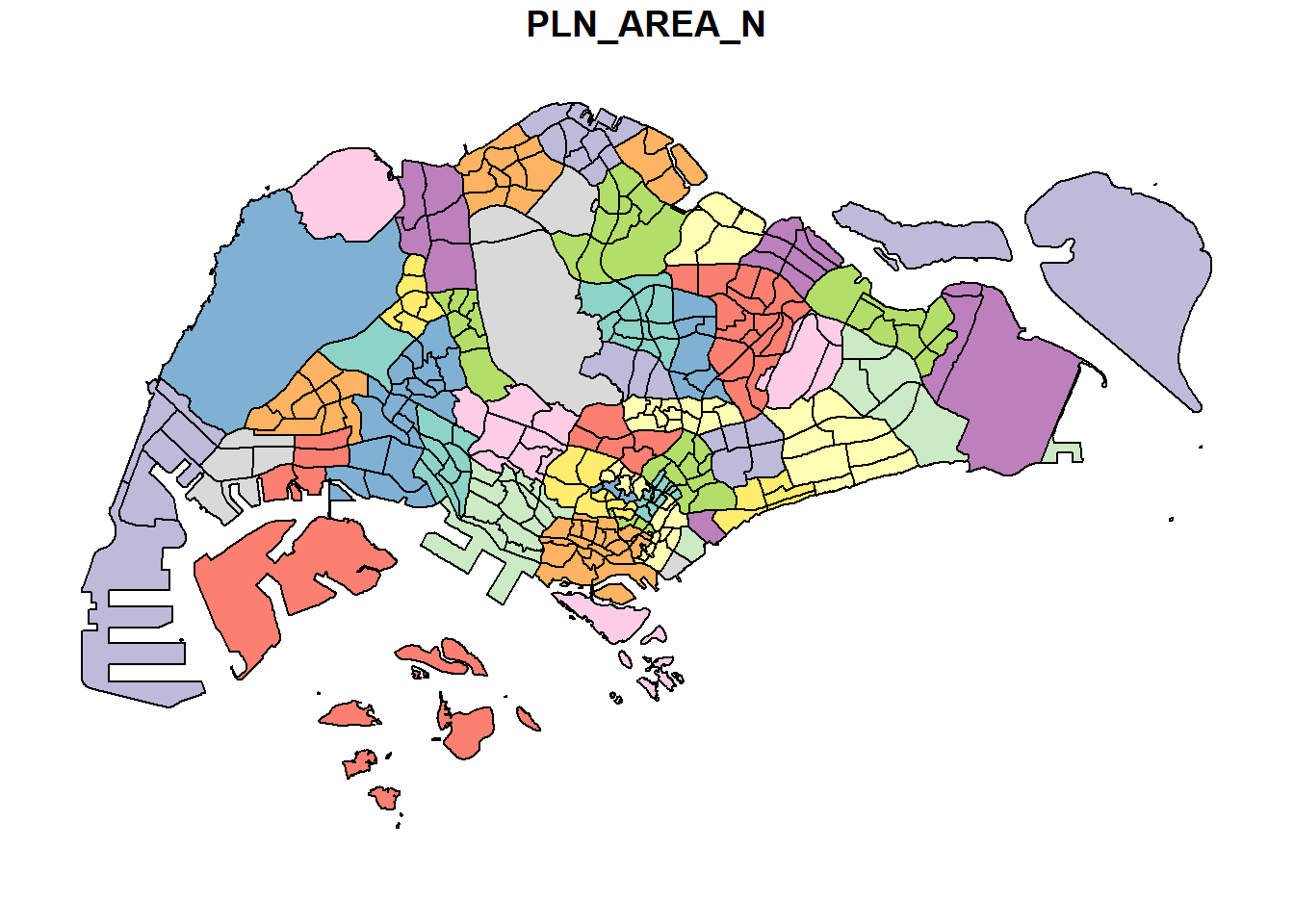
plot(mpsz["PLN_AREA_C"])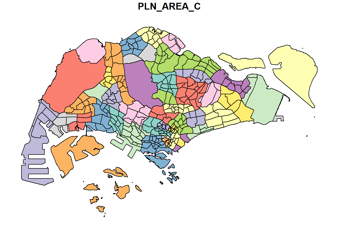
plot(mpsz["REGION_C"])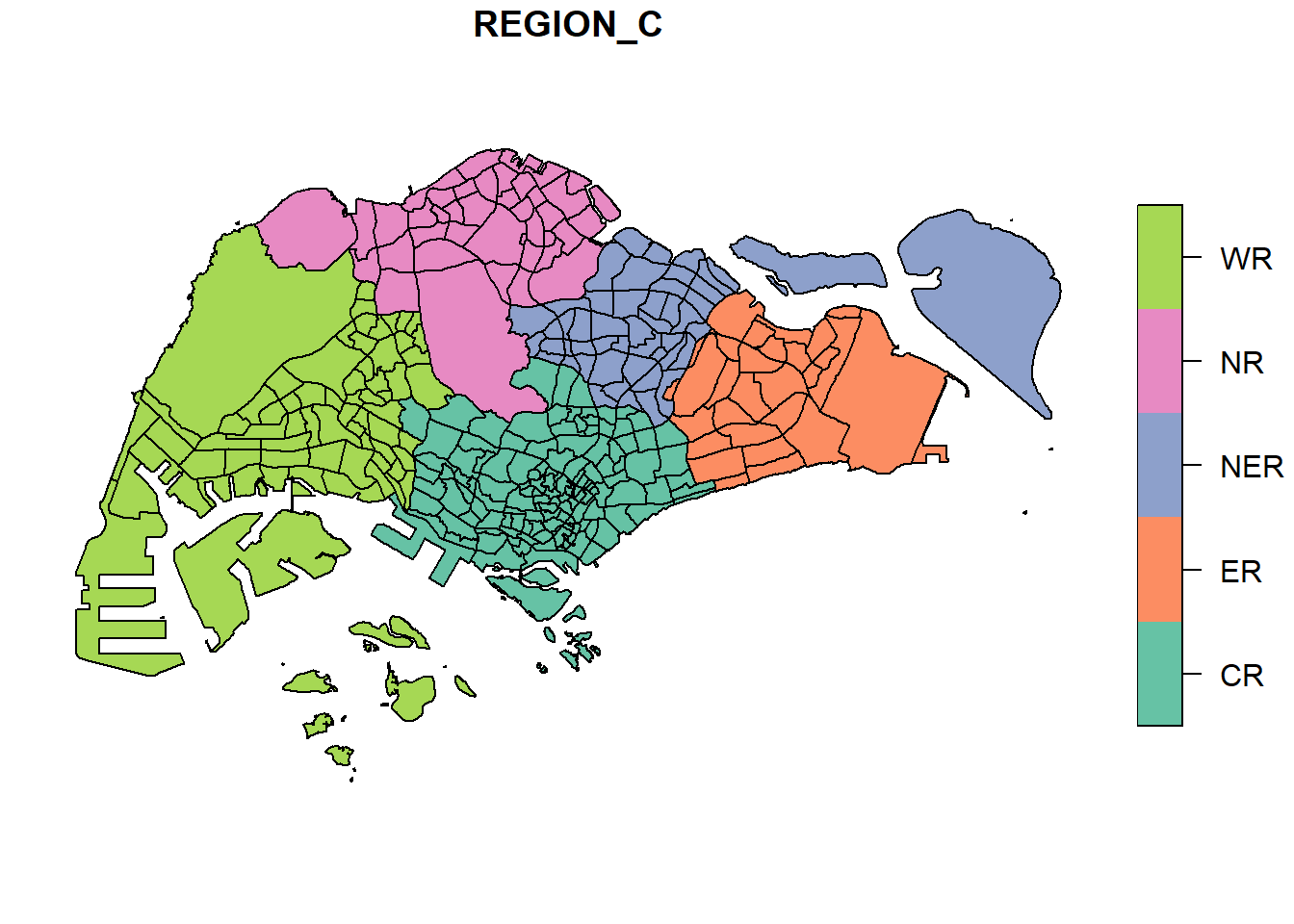
Note: plot() is meant for plotting the geospatial object for quick observation. For a high cartographic quality plot, other R package such as tmap should be used.
1.7 Working with Projection
Map projection is an important property of a geospatial data. In order to perform geoprocessing using two geospatial data, both geospatial data have to be projected using similar coordinate system.
In this section, it will illustrate how to project a simple feature data frame from one coordinate system to another coordinate system. The technical term of this process is called projection transformation.
1.7.1 Assigning EPSG code to a simple feature data frame
A common issue that can happen during importing process of geospatial data into R is that the coordinate system of the source data was either missing (such as due to missing .proj for ESRI shapefile) or wrongly assigned during the importing process.
This is an example the coordinate system of mpsz simple feature data frame by using st_crs() of sf package as shown in the code chunk below.
st_crs(mpsz)Coordinate Reference System:
User input: SVY21
wkt:
PROJCRS["SVY21",
BASEGEOGCRS["SVY21[WGS84]",
DATUM["World Geodetic System 1984",
ELLIPSOID["WGS 84",6378137,298.257223563,
LENGTHUNIT["metre",1]],
ID["EPSG",6326]],
PRIMEM["Greenwich",0,
ANGLEUNIT["Degree",0.0174532925199433]]],
CONVERSION["unnamed",
METHOD["Transverse Mercator",
ID["EPSG",9807]],
PARAMETER["Latitude of natural origin",1.36666666666667,
ANGLEUNIT["Degree",0.0174532925199433],
ID["EPSG",8801]],
PARAMETER["Longitude of natural origin",103.833333333333,
ANGLEUNIT["Degree",0.0174532925199433],
ID["EPSG",8802]],
PARAMETER["Scale factor at natural origin",1,
SCALEUNIT["unity",1],
ID["EPSG",8805]],
PARAMETER["False easting",28001.642,
LENGTHUNIT["metre",1],
ID["EPSG",8806]],
PARAMETER["False northing",38744.572,
LENGTHUNIT["metre",1],
ID["EPSG",8807]]],
CS[Cartesian,2],
AXIS["(E)",east,
ORDER[1],
LENGTHUNIT["metre",1,
ID["EPSG",9001]]],
AXIS["(N)",north,
ORDER[2],
LENGTHUNIT["metre",1,
ID["EPSG",9001]]]]Although the mpsz data frame is projected in svy21 but upon examination at the end of the print, it indicates that the EPSG is 9001. This is a wrong EPSG code because the correct EPSG code for svy21 should be 3414.
In order to assign the correct EPSG code to the mpsz data frame, st_set_crs() of sf package is used as shown in the code chunk below.
mpsz3414 <- st_set_crs(mpsz, 3414)Now, to inspect the CSR again by using the code chunk below.
st_crs(mpsz3414)Coordinate Reference System:
User input: EPSG:3414
wkt:
PROJCRS["SVY21 / Singapore TM",
BASEGEOGCRS["SVY21",
DATUM["SVY21",
ELLIPSOID["WGS 84",6378137,298.257223563,
LENGTHUNIT["metre",1]]],
PRIMEM["Greenwich",0,
ANGLEUNIT["degree",0.0174532925199433]],
ID["EPSG",4757]],
CONVERSION["Singapore Transverse Mercator",
METHOD["Transverse Mercator",
ID["EPSG",9807]],
PARAMETER["Latitude of natural origin",1.36666666666667,
ANGLEUNIT["degree",0.0174532925199433],
ID["EPSG",8801]],
PARAMETER["Longitude of natural origin",103.833333333333,
ANGLEUNIT["degree",0.0174532925199433],
ID["EPSG",8802]],
PARAMETER["Scale factor at natural origin",1,
SCALEUNIT["unity",1],
ID["EPSG",8805]],
PARAMETER["False easting",28001.642,
LENGTHUNIT["metre",1],
ID["EPSG",8806]],
PARAMETER["False northing",38744.572,
LENGTHUNIT["metre",1],
ID["EPSG",8807]]],
CS[Cartesian,2],
AXIS["northing (N)",north,
ORDER[1],
LENGTHUNIT["metre",1]],
AXIS["easting (E)",east,
ORDER[2],
LENGTHUNIT["metre",1]],
USAGE[
SCOPE["Cadastre, engineering survey, topographic mapping."],
AREA["Singapore - onshore and offshore."],
BBOX[1.13,103.59,1.47,104.07]],
ID["EPSG",3414]]Notice that the EPSG code is 3414 now.
1.7.2 Transforming the projection of preschool from wgs84 to svy21
In geospatial analytics, it is very common to transform the original data from geographic coordinate system to projected coordinate system. This is because geographic coordinate system is not appropriate if the analysis requires the use of distance or/and area measurements.
Examining the preschool simple feature data frame as an example. The print below reveals that it is in wgs84 coordinate system.
st_geometry(preschool)Geometry set for 2290 features
Geometry type: POINT
Dimension: XYZ
Bounding box: xmin: 103.6878 ymin: 1.247759 xmax: 103.9897 ymax: 1.462134
z_range: zmin: 0 zmax: 0
Geodetic CRS: WGS 84
First 5 geometries:Hence, this is a scenario that illustrates st_set_crs() is not appropriate and st_transform() of sf package should be used.
This is due to the fact that a re-projection is needed for preschool from one coordinate system to another coordinate system mathematically.
The projection transformation is performed by using the code chunk below.
preschool3414 <- st_transform(preschool,
                              crs = 3414)
Note: In practice, we will need to find out the appropriate project coordinate system to use before performing the projection transformation.
The content of preschool3414 sf data frame is displayed again with the code chunk below:
st_geometry(preschool3414)Geometry set for 2290 features
Geometry type: POINT
Dimension: XYZ
Bounding box: xmin: 11810.03 ymin: 25596.33 xmax: 45404.24 ymax: 49300.88
z_range: zmin: 0 zmax: 0
Projected CRS: SVY21 / Singapore TM
First 5 geometries:
Note
Notice that it is in svy21 projected coordinate system now. Furthermore, referencing to Bounding box:, the values are greater than 0-360 range of decimal degree commonly used by most of the geographic coordinate systems.
1.8 Importing and Converting An Aspatial Data
In practice, it is not unusual that we will come across data such as listing of Inside Airbnb. We call this kind of data aspatial data. Mainly because it is not a geospatial data but among the data fields, there are two fields that capture the x- and y-coordinates of the data points.
In this section, it will illustrate how to import an aspatial data into R environment and save it as a tibble data frame. Next, it will be converted it into a simple feature data frame.
For the purpose of this exercise, the listings.csv data downloaded from AirBnb will be used.
1.8.1 Importing the aspatial data
Since listings data set is in csv file format, read_csv() of readr package will be used to import listing.csv as shown in the code chunk below. The output R object is called listings and it is a tibble data frame.
listings <- read_csv("data/aspatial/listings.csv")After importing the data file into R, it is important to examine if the data file has been imported correctly.
The code chunk below shows list() of Base R instead of glimpse() to do the job.
list(listings)[[1]]
# A tibble: 3,540 × 18
id name host_id host_name neighbourhood_group neighbourhood latitude
<dbl> <chr> <dbl> <chr> <chr> <chr> <dbl>
1 71609 Ensuite … 367042 Belinda East Region Tampines 1.35
2 71896 B&B Roo… 367042 Belinda East Region Tampines 1.35
3 71903 Room 2-n… 367042 Belinda East Region Tampines 1.35
4 275343 10min wa… 1439258 Kay Central Region Bukit Merah 1.29
5 275344 15 mins … 1439258 Kay Central Region Bukit Merah 1.29
6 289234 Booking … 367042 Belinda East Region Tampines 1.34
7 294281 5 mins w… 1521514 Elizabeth Central Region Newton 1.31
8 324945 Comforta… 1439258 Kay Central Region Bukit Merah 1.29
9 330095 Relaxing… 1439258 Kay Central Region Bukit Merah 1.29
10 344803 Budget s… 367042 Belinda East Region Tampines 1.35
# ℹ 3,530 more rows
# ℹ 11 more variables: longitude <dbl>, room_type <chr>, price <dbl>,
# minimum_nights <dbl>, number_of_reviews <dbl>, last_review <date>,
# reviews_per_month <dbl>, calculated_host_listings_count <dbl>,
# availability_365 <dbl>, number_of_reviews_ltm <dbl>, license <chr>The output reveals that listing tibble data frame consists of 3540 rows and 18 columns. Two useful fields we are going to use in the next phase are latitude and longitude. Note that they are in decimal degree format. As a best guess, the assumption is that the data is in wgs84 Geographic Coordinate System.
1.8.2 Creating a simple feature data frame from an aspatial data frame
The code chunk below converts listing data frame into a simple feature data frame by using st_as_sf() of sf packages
listings_sf <- st_as_sf(listings,
                        coords = c("longitude", "latitude"),
                        crs = 4326) %>%
  st_transform(crs = 3414)
Things to learn from the arguments above:
- coords argument requires you to provide the column name of the x-coordinates first then followed by the column name of the y-coordinates.
- crs argument requires you to provide the coordinates system in epsg format. EPSG: 4326 is wgs84 Geographic Coordinate System and EPSG: 3414 is Singapore SVY21 Projected Coordinate System. You can search for other country’s ESPG code by referring to epsg.io.
- %>% is used to nest st_transform() to transform the newly created simple feature data frame into svy21 projected coordinates system.
Now to examine the content of this newly created listings_sf simple feature data frame.
glimpse(listings_sf)Rows: 3,540
Columns: 17
$ id <dbl> 71609, 71896, 71903, 275343, 275344, 28…
$ name <chr> "Ensuite Room (Room 1 & 2) near EXPO", …
$ host_id <dbl> 367042, 367042, 367042, 1439258, 143925…
$ host_name <chr> "Belinda", "Belinda", "Belinda", "Kay",…
$ neighbourhood_group <chr> "East Region", "East Region", "East Reg…
$ neighbourhood <chr> "Tampines", "Tampines", "Tampines", "Bu…
$ room_type <chr> "Private room", "Private room", "Privat…
$ price <dbl> NA, 80, 80, 50, 50, NA, 85, 65, 45, 54,…
$ minimum_nights <dbl> 92, 92, 92, 180, 180, 92, 92, 180, 180,…
$ number_of_reviews <dbl> 19, 24, 46, 20, 16, 12, 131, 17, 5, 60,…
$ last_review <date> 2020-01-17, 2019-10-13, 2020-01-09, 20…
$ reviews_per_month <dbl> 0.12, 0.15, 0.29, 0.15, 0.11, 0.08, 0.8…
$ calculated_host_listings_count <dbl> 6, 6, 6, 49, 49, 6, 7, 49, 49, 6, 7, 7,…
$ availability_365 <dbl> 89, 148, 90, 62, 0, 88, 365, 0, 0, 365,…
$ number_of_reviews_ltm <dbl> 0, 0, 0, 0, 2, 0, 0, 1, 1, 1, 0, 0, 0, …
$ license <chr> NA, NA, NA, "S0399", "S0399", NA, NA, "…
$ geometry <POINT [m]> POINT (41972.5 36390.05), POINT (…Table above shows the content of listing_sf. Notice that a new column called geometry has been added into the data frame. On the other hand, the longitude and latitude columns have been dropped from the data frame.
1.9 Geoprocessing with sf package
Besides providing functions to handle (i.e. importing, exporting, assigning projection, transforming projection) geospatial data, sf package also offers a wide range of geoprocessing (also known as GIS analysis) functions.
In this section, it will provide learning on how to perform two commonly used geoprocessing functions, namely buffering and point in polygon count.
1.9.1 Buffering
The scenario:
The authority is planning to upgrade the exiting cycling path. To do so, they need to acquire 5 metres of reserved land on both sides of the current cycling path. You are tasked to determine the extend of the land need to be acquired and their total area.
The solution:
Firstly, st_buffer() of sf package is used to compute the 5-meter buffers around cycling paths
buffer_cycling <- st_buffer(cyclingpath,
                            dist = 5, nQuadSegs = 30)
This is followed by calculating the area of the buffers as shown in the code chunk below:
buffer_cycling$AREA <- st_area(buffer_cycling)Lastly, sum() of Base R will be used to derive the total land involved
sum(buffer_cycling$AREA)2218855 [m^2]Task Accomplished!
1.9.2 Point-in-polygon count
The scenario:
A pre-school service group want to find out the number of pre-schools in each Planning Subzone.
The solution:
The code chunk below performs two operations at once. Firstly, identifying pre-schools located inside each Planning Subzone by using st_intersects(). Next, length() of Base R is used to calculate numbers of pre-schools that fall inside each planning subzone.
mpsz3414$`PreSch Count` <- lengths(st_intersects(mpsz3414, preschool3414))Warning: This should not confused with st_intersection().
The summary statistics of the newly derived PreSch Count field can be checked by using summary() as shown in the code chunk below.
summary(mpsz3414$`PreSch Count`) Min. 1st Qu. Median Mean 3rd Qu. Max.
0.00 0.00 4.00 7.09 10.00 72.00 To list the planning subzone with the most number of pre-schools, the top_n() of dplyr package is used as shown in the code chunk below.
top_n(mpsz3414, 1, `PreSch Count`)Simple feature collection with 1 feature and 16 fields
Geometry type: MULTIPOLYGON
Dimension: XY
Bounding box: xmin: 39655.33 ymin: 35966 xmax: 42940.57 ymax: 38622.37
Projected CRS: SVY21 / Singapore TM
OBJECTID SUBZONE_NO SUBZONE_N SUBZONE_C CA_IND PLN_AREA_N PLN_AREA_C
1 189 2 TAMPINES EAST TMSZ02 N TAMPINES TM
REGION_N REGION_C INC_CRC FMEL_UPD_D X_ADDR Y_ADDR SHAPE_Leng
1 EAST REGION ER 21658EAAF84F4D8D 2014-12-05 41122.55 37392.39 10180.62
SHAPE_Area geometry PreSch Count
1 4339824 MULTIPOLYGON (((42196.76 38... 72Attempt: Calculate the density of pre-school by planning subzone.
The solution:
Firstly, the code chunk below uses st_area() of sf package to derive the area of each planning subzone.
mpsz3414$Area <- mpsz3414 %>%
  st_area()
Next, mutate() of dplyr package is used to compute the density by using the code chunk below:
mpsz3414 <- mpsz3414 %>%
  mutate(`PreSch Density` = `PreSch Count`/Area * 1000000)
Similarly, the planning subzone with the highest density of pre-schools can be listed using the top_n() of dplyr package is used as shown in the code chunk below.
top_n(mpsz3414, 1, `PreSch Density`)Simple feature collection with 1 feature and 18 fields
Geometry type: MULTIPOLYGON
Dimension: XY
Bounding box: xmin: 29501.64 ymin: 28623.75 xmax: 29976.93 ymax: 29362.03
Projected CRS: SVY21 / Singapore TM
OBJECTID SUBZONE_NO SUBZONE_N SUBZONE_C CA_IND PLN_AREA_N PLN_AREA_C
1 27 8 CECIL DTSZ08 Y DOWNTOWN CORE DT
REGION_N REGION_C INC_CRC FMEL_UPD_D X_ADDR Y_ADDR
1 CENTRAL REGION CR 65AA82AF6F4D925D 2014-12-05 29730.2 29011.33
SHAPE_Leng SHAPE_Area geometry PreSch Count
1 2116.095 196619.9 MULTIPOLYGON (((29808.18 28... 7
Area PreSch Density
1 196619.9 [m^2] 35.60169 [1/m^2]1.10 Exploratory Data Analysis (EDA)
In practice, most geospatial analytics start with Exploratory Data Analysis(EDA). In this section, it demonstrates how to use appropriate ggplot2 functions to create functional and yet truthful statistical graphs for EDA purposes.
Firstly, we will plot a histogram to reveal the distribution of PreSch Density. Conventionally, hist() of R Graphics will be used as shown in the code chunk below.
hist(mpsz3414$`PreSch Density`)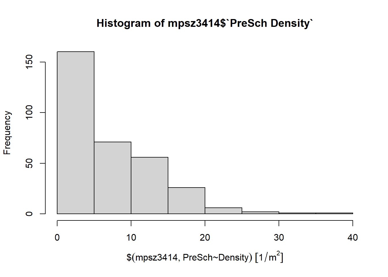
Although the syntax is very easy to use the output however, is far from meeting publication quality. Furthermore, the function has limited room for further customisation.
In the code chunk below, appropriate ggplot2 functions will be used.
ggplot(data = mpsz3414,
       aes(x = as.numeric(`PreSch Density`))) +
  geom_histogram(bins = 20,
                 color = "black",
                 fill = "light blue") +
  labs(title = "Are pre-schools evenly distributed in Singapore ?",
       subtitle = "There are many planning sub-zones with a single pre-school, on the other hand, \nthere are two planning sub-zones with at least 20 pre-schools",
       x = "Pre-school density (per km sq)",
       y = "Frequency")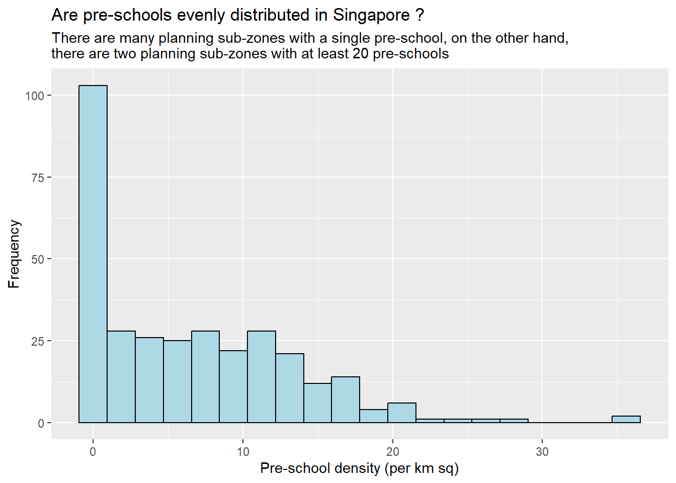
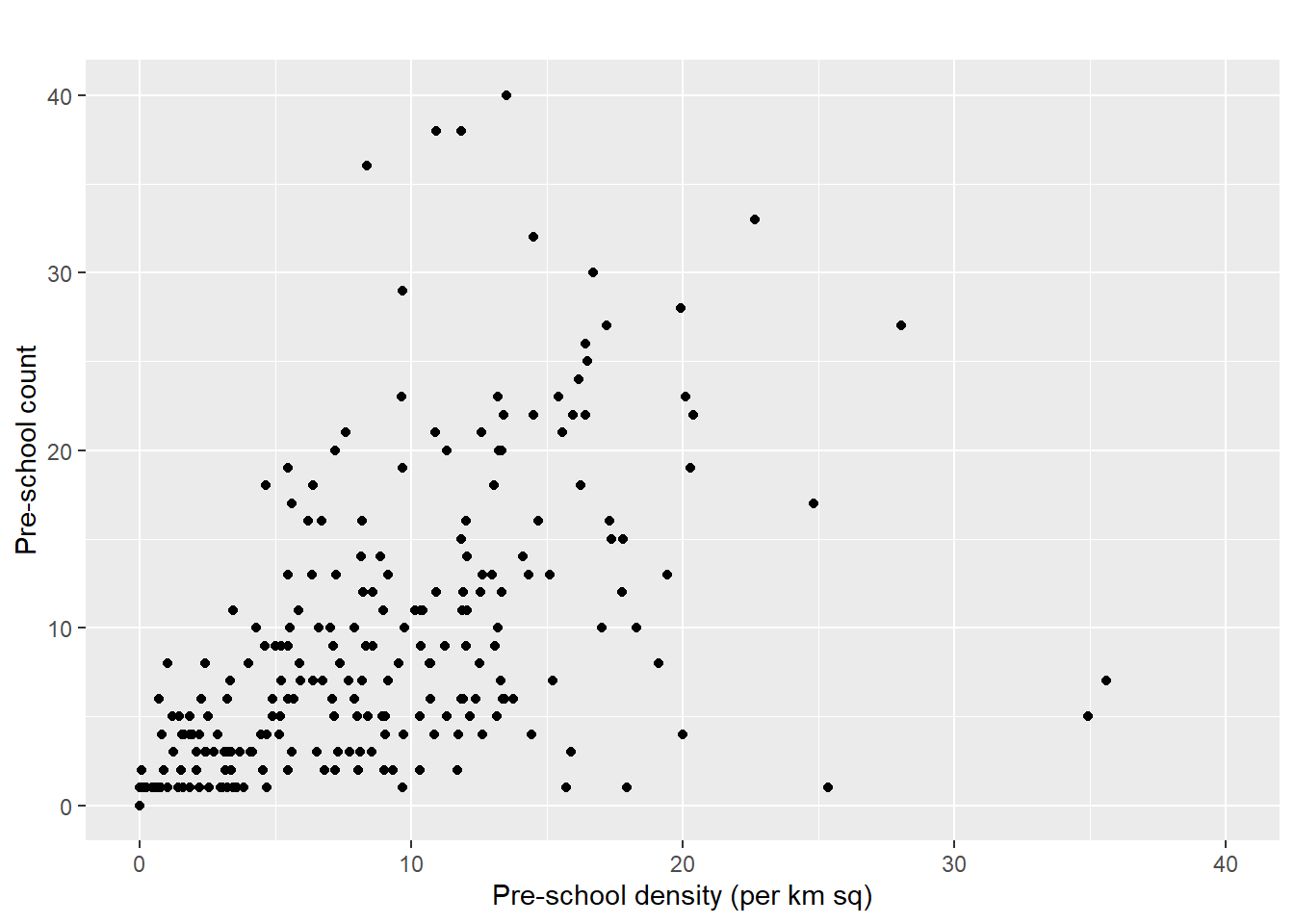
Attempt: Using ggplot2 method, plot a scatterplot showing the relationship between Pre-school Density and Pre-school Count.
ggplot(data = mpsz3414,
       aes(y = `PreSch Count`,
           x = as.numeric(`PreSch Density`))) +
  geom_point(color = "black",
             fill = "light blue") +
  xlim(0, 40) +
  ylim(0, 40) +
  labs(title = "",
      y = "Pre-school count",
      x = "Pre-school density (per km sq)")