pacman::p_load(spdep, sf, tmap, tidyverse, knitr)Hands-on Exercise 4: Spatial Weights and Applications
1 Spatial Weights and Applications
1.1 Overview
In this hands-on exercise, it will run through the process of computing spatial weights using R. By the end to this hands-on exercise, one should be able to:
- import geospatial data using appropriate function(s) of sf package,
- import csv file using appropriate function of readr package,
- perform relational join using appropriate join function of dplyr package,
- compute spatial weights using appropriate functions of spdep package, and
- calculate spatially lagged variables using appropriate functions of spdep package.
1.2 The Study Area and Data
Two data sets will be used in this hands-on exercise, they are:
Hunan county boundary layer. This is a geospatial data set in ESRI shapefile format.Hunan_2012.csv; This csv file contains selected Hunan’s local development indicators in 2012.
1.2.1 Getting Started
Before getting started, ensure that spdep, sf, tmap, tidyverse and knitrpackages of R are currently installed in R.
1.3 Getting the Data into the R environment
In this section, the geospatial data and its associated attribute table will be brought in R environment. The geospatial data is in ESRI shapefile format and the attribute table is in csv format.
1.3.1 Importing shapefile in R environment
The code chunk below uses st_read() of sf package to import Hunan shapefile into R. The imported shapefile will be a simple feature Object of sf.
hunan <- st_read(dsn = "data/geospatial",
                 layer = "Hunan")
Reading layer `Hunan' from data source
`C:\zjho008\ISSS626-GAA\Hands-on_Ex\Hands-on_Ex04\data\geospatial'
using driver `ESRI Shapefile'
Simple feature collection with 88 features and 7 fields
Geometry type: POLYGON
Dimension: XY
Bounding box: xmin: 108.7831 ymin: 24.6342 xmax: 114.2544 ymax: 30.12812
Geodetic CRS: WGS 841.3.2 Importing csv file into R environment
Next, Hunan_2012.csv will be imported into R by using read_csv() of readr package. The output is a R dataframe class.
hunan2012 <- read_csv("data/aspatial/Hunan_2012.csv")Rows: 88 Columns: 29
── Column specification ────────────────────────────────────────────────────────
Delimiter: ","
chr (2): County, City
dbl (27): avg_wage, deposite, FAI, Gov_Rev, Gov_Exp, GDP, GDPPC, GIO, Loan, ...
ℹ Use `spec()` to retrieve the full column specification for this data.
ℹ Specify the column types or set `show_col_types = FALSE` to quiet this message.1.3.3 Performing relational join
The code chunk below will be used to update the attribute table of hunan’s SpatialPolygonsDataFrame with the attribute fields of hunan2012 dataframe. This is performed by using left_join() of dplyr package.
The select() function is used to select variables that are objectively used for the spatial analysis.
hunan <- left_join(hunan, hunan2012) %>%
  select(1:4, 7, 15)
Joining with `by = join_by(County)`1.4 Visualising Regional Development Indicator
Now, a basemap and a choropleth map will be prepared showing the distribution of GDPPC 2012 by using qtm() of tmap package.
basemap <- tm_shape(hunan) +
  tm_polygons() +
  tm_text("NAME_3", size = 0.5)

gdppc <- qtm(hunan, "GDPPC")
tmap_arrange(basemap, gdppc, asp = 1, ncol = 2)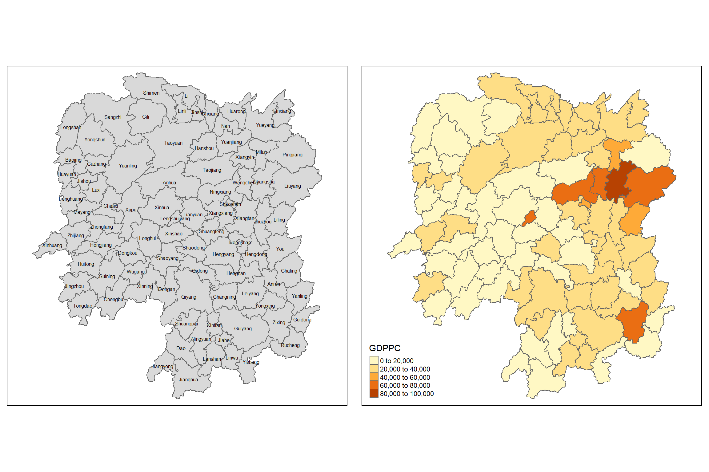
Note: Gross Domestic Product per Capita (GDPPC)
1.5 Computing Contiguity Spatial Weights
In this section, we will learn how to use poly2nb() of spdep package to compute contiguity weight matrices for the study area.
This function builds a neighbours list based on regions with contiguous boundaries. From the documentation, we learn that we can pass a “queen” argument that takes TRUE or FALSE as options. If this argument is not specified the argument’s default is set to TRUE, that is, if we don’t specify queen = FALSE this function will return a list of first order neighbours using the Queen criteria.
1.5.1 Computing (QUEEN) contiguity based neighbours
The code chunk below is used to compute Queen contiguity weight matrix.
wm_q <- poly2nb(hunan, queen = TRUE)
summary(wm_q)
Neighbour list object:
Number of regions: 88
Number of nonzero links: 448
Percentage nonzero weights: 5.785124
Average number of links: 5.090909
Link number distribution:
1 2 3 4 5 6 7 8 9 11
2 2 12 16 24 14 11 4 2 1
2 least connected regions:
30 65 with 1 link
1 most connected region:
85 with 11 linksThe summary report above shows that there are 88 area units (regions) in Hunan. The most connected area unit has 11 neighbours. There are two area units with only one neighbour.
For each polygon in the polygon object, wm_q lists all neighbouring polygons. For example, to see the neighbours for the first polygon in the object, type:
wm_q[[1]][1] 2 3 4 57 85Polygon 1 has 5 neighbours. The numbers represent the polygon IDs as stored in hunan SpatialPolygonsDataFrame class.
We can retrieve the county name of Polygon ID=1 by using the code chunk below:
hunan$County[1][1] "Anxiang"The output reveals that Polygon ID=1 is Anxiang county.
To reveal the county names of the five neighbouring polygons, the code chunk will be used:
hunan$NAME_3[c(2,3,4,57,85)][1] "Hanshou" "Jinshi" "Li" "Nan" "Taoyuan"We can retrieve the GDPPC of these five counties by using the code chunk below.
nb1 <- wm_q[[1]]
nb1 <- hunan$GDPPC[nb1]
nb1
[1] 20981 34592 24473 21311 22879The printed output above shows that the GDPPC of the five nearest neighbours based on Queen’s method are 20981, 34592, 24473, 21311 and 22879 respectively.
We can display the complete weight matrix by using str().
str(wm_q)List of 88
$ : int [1:5] 2 3 4 57 85
$ : int [1:5] 1 57 58 78 85
$ : int [1:4] 1 4 5 85
$ : int [1:4] 1 3 5 6
$ : int [1:4] 3 4 6 85
$ : int [1:5] 4 5 69 75 85
$ : int [1:4] 67 71 74 84
$ : int [1:7] 9 46 47 56 78 80 86
$ : int [1:6] 8 66 68 78 84 86
$ : int [1:8] 16 17 19 20 22 70 72 73
$ : int [1:3] 14 17 72
$ : int [1:5] 13 60 61 63 83
$ : int [1:4] 12 15 60 83
$ : int [1:3] 11 15 17
$ : int [1:4] 13 14 17 83
$ : int [1:5] 10 17 22 72 83
$ : int [1:7] 10 11 14 15 16 72 83
$ : int [1:5] 20 22 23 77 83
$ : int [1:6] 10 20 21 73 74 86
$ : int [1:7] 10 18 19 21 22 23 82
$ : int [1:5] 19 20 35 82 86
$ : int [1:5] 10 16 18 20 83
$ : int [1:7] 18 20 38 41 77 79 82
$ : int [1:5] 25 28 31 32 54
$ : int [1:5] 24 28 31 33 81
$ : int [1:4] 27 33 42 81
$ : int [1:3] 26 29 42
$ : int [1:5] 24 25 33 49 54
$ : int [1:3] 27 37 42
$ : int 33
$ : int [1:8] 24 25 32 36 39 40 56 81
$ : int [1:8] 24 31 50 54 55 56 75 85
$ : int [1:5] 25 26 28 30 81
$ : int [1:3] 36 45 80
$ : int [1:6] 21 41 47 80 82 86
$ : int [1:6] 31 34 40 45 56 80
$ : int [1:4] 29 42 43 44
$ : int [1:4] 23 44 77 79
$ : int [1:5] 31 40 42 43 81
$ : int [1:6] 31 36 39 43 45 79
$ : int [1:6] 23 35 45 79 80 82
$ : int [1:7] 26 27 29 37 39 43 81
$ : int [1:6] 37 39 40 42 44 79
$ : int [1:4] 37 38 43 79
$ : int [1:6] 34 36 40 41 79 80
$ : int [1:3] 8 47 86
$ : int [1:5] 8 35 46 80 86
$ : int [1:5] 50 51 52 53 55
$ : int [1:4] 28 51 52 54
$ : int [1:5] 32 48 52 54 55
$ : int [1:3] 48 49 52
$ : int [1:5] 48 49 50 51 54
$ : int [1:3] 48 55 75
$ : int [1:6] 24 28 32 49 50 52
$ : int [1:5] 32 48 50 53 75
$ : int [1:7] 8 31 32 36 78 80 85
$ : int [1:6] 1 2 58 64 76 85
$ : int [1:5] 2 57 68 76 78
$ : int [1:4] 60 61 87 88
$ : int [1:4] 12 13 59 61
$ : int [1:7] 12 59 60 62 63 77 87
$ : int [1:3] 61 77 87
$ : int [1:4] 12 61 77 83
$ : int [1:2] 57 76
$ : int 76
$ : int [1:5] 9 67 68 76 84
$ : int [1:4] 7 66 76 84
$ : int [1:5] 9 58 66 76 78
$ : int [1:3] 6 75 85
$ : int [1:3] 10 72 73
$ : int [1:3] 7 73 74
$ : int [1:5] 10 11 16 17 70
$ : int [1:5] 10 19 70 71 74
$ : int [1:6] 7 19 71 73 84 86
$ : int [1:6] 6 32 53 55 69 85
$ : int [1:7] 57 58 64 65 66 67 68
$ : int [1:7] 18 23 38 61 62 63 83
$ : int [1:7] 2 8 9 56 58 68 85
$ : int [1:7] 23 38 40 41 43 44 45
$ : int [1:8] 8 34 35 36 41 45 47 56
$ : int [1:6] 25 26 31 33 39 42
$ : int [1:5] 20 21 23 35 41
$ : int [1:9] 12 13 15 16 17 18 22 63 77
$ : int [1:6] 7 9 66 67 74 86
$ : int [1:11] 1 2 3 5 6 32 56 57 69 75 ...
$ : int [1:9] 8 9 19 21 35 46 47 74 84
$ : int [1:4] 59 61 62 88
$ : int [1:2] 59 87
- attr(*, "class")= chr "nb"
- attr(*, "region.id")= chr [1:88] "1" "2" "3" "4" ...
- attr(*, "call")= language poly2nb(pl = hunan, queen = TRUE)
- attr(*, "type")= chr "queen"
- attr(*, "sym")= logi TRUE
Warning
Be warned: The output might cut across several pages. Do consider saving the trees if you are going to print out the report.
1.5.1.1 DIY
wm_q[[30]][1] 33wm_q[[65]][1] 76wm_q[[85]] [1] 1 2 3 5 6 32 56 57 69 75 78hunan$County[85][1] "Taoyuan"To reveal the county names of the eleven neighbouring polygons, the code chunk will be used:
hunan$NAME_3[c(1,2,3,5,6,32,56,57,69,75,78)] [1] "Anxiang" "Hanshou" "Jinshi" "Linli" "Shimen" "Yuanling"
[7] "Anhua" "Nan" "Cili" "Sangzhi" "Taojiang"Revealing the GDPPC of there eleven counties by using the code chunk below.
nb1 <- wm_q[[85]]
nb1 <- hunan$GDPPC[nb1]
nb1
[1] 23667 20981 34592 25554 27137 24194 14567 21311 18714 14624 195091.5.2 Creating (ROOK) contiguity based neighbours
The code chunk below is used to compute Rook contiguity weight matrix.
wm_r <- poly2nb(hunan, queen = FALSE)
summary(wm_r)
Neighbour list object:
Number of regions: 88
Number of nonzero links: 440
Percentage nonzero weights: 5.681818
Average number of links: 5
Link number distribution:
1 2 3 4 5 6 7 8 9 10
2 2 12 20 21 14 11 3 2 1
2 least connected regions:
30 65 with 1 link
1 most connected region:
85 with 10 linksThe summary report above shows that there are 88 area units in Hunan. The most connected area unit has 10 neighbours. There are two area units with only one neighbours.
1.5.3 Visualising contiguity weights
A connectivity graph takes a point and displays a line to each neighbouring point. We are working with polygons at the moment, so we will need to get points in order to make our connectivity graphs. The most typically used method for this will be polygon centroids. We will calculate these in the sf package before moving onto the graphs. Getting Latitude and Longitude of Polygon Centroids
We will need points to associate with each polygon before we can make our connectivity graph. It will be a little more complicated than just running st_centroid on the sf object: us.bound. We need the coordinates in a separate data frame for this to work. To do this we will use a mapping function. The mapping function applies a given function to each element of a vector and returns a vector of the same length. Our input vector will be the geometry column of us.bound. Our function will be st_centroid. We will be using map_dbl variation of map from the purrr package. For more documentation, check out map documentation
To get our longitude values we map the st_centroid function over the geometry column of us.bound and access the longitude value through double bracket notation [[]] and 1. This allows us to get only the longitude, which is the first value in each centroid.
longitude <- map_dbl(hunan$geometry, ~st_centroid(.x)[[1]])We can do the same for latitude with one key difference. We access the second value per each centroid with [[2]].
latitude <- map_dbl(hunan$geometry, ~st_centroid(.x)[[2]])Now that longitude and latitude is obtained, we use cbind to put longitude and latitude into the same object.
coords <- cbind(longitude, latitude)Upon running the code chunk, we can check the first few observations to see if things are formatted correctly.
head(coords) longitude latitude
[1,] 112.1531 29.44362
[2,] 112.0372 28.86489
[3,] 111.8917 29.47107
[4,] 111.7031 29.74499
[5,] 111.6138 29.49258
[6,] 111.0341 29.798631.5.3.1 Plotting Queen contiguity based neighbours map
plot(hunan$geometry, border = "lightgrey")
plot(wm_q, coords, pch = 19, cex = 0.6, add = TRUE, col = "red")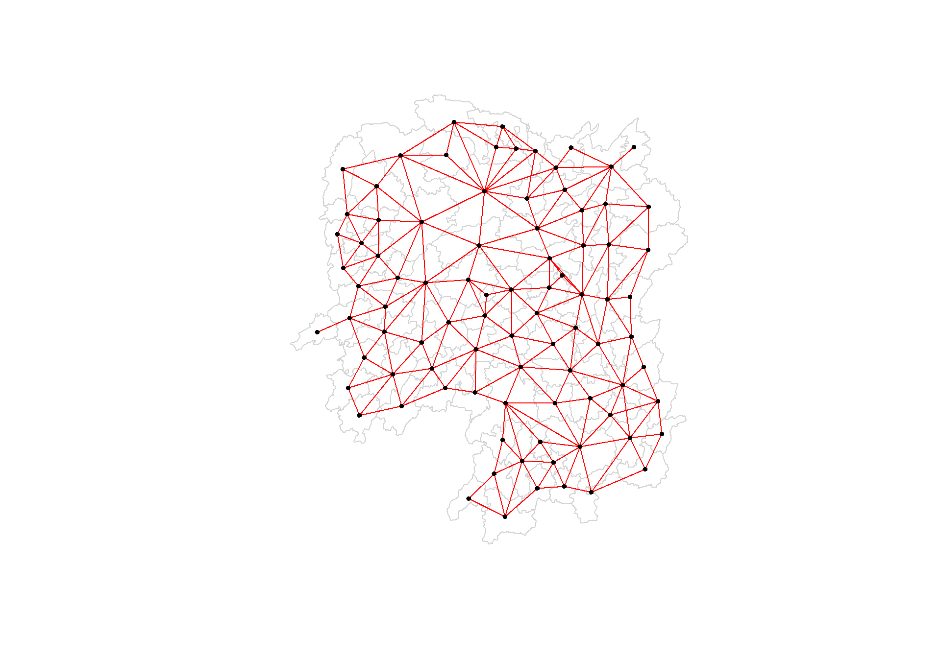
1.5.3.2 Plotting Rook contiguity based neighbours map
plot(hunan$geometry, border = "lightgrey")
plot(wm_r, coords, pch = 19, cex = 0.6, add = TRUE, col = "red")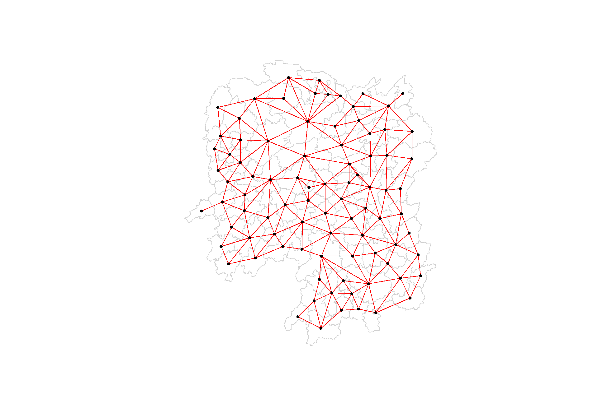
1.5.3.3 Plotting both Queen and Rook contiguity based neighbours maps
par(mfrow = c(1,2))
plot(hunan$geometry, border = "lightgrey", main = "Queen Contiguity")
plot(wm_q, coords, pch = 19, cex = 0.6, add = TRUE, col = "red")
plot(hunan$geometry, border = "lightgrey", main = "Rook Contiguity")
plot(wm_r, coords, pch = 19, cex = 0.6, add = TRUE, col = "red")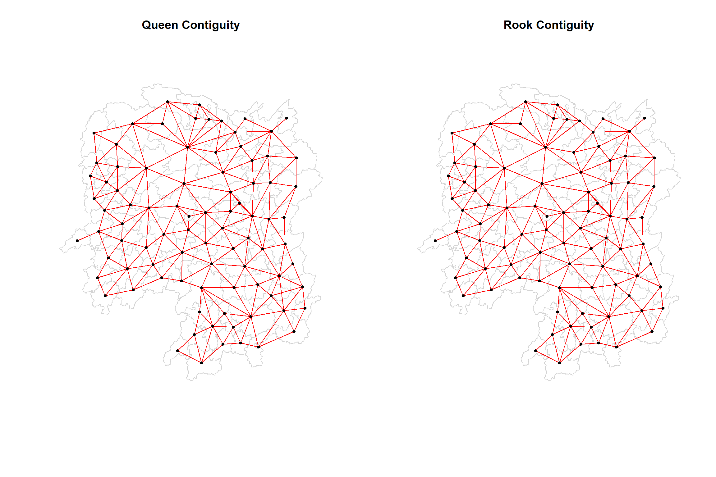
1.6 Computing distance based neighbours
In this section, we will learn how to derive distance-based weight matrices by using dnearneigh() of spdep package.
The function identifies neighbours of region points by Euclidean distance with a distance band with lower d1= and upper d2= bounds controlled by the bounds = argument. If un-projected coordinates are used and either specified in the coordinates object x or with x as a two column matrix and = TRUE, great circle distances in km will be calculated assuming the WGS84 reference ellipsoid.
1.6.1 Determine the cut-off distance
Firstly, we need to determine the upper limit for distance band by using the steps below:
- Return a matrix with the indices of points belonging to the set of the k nearest neighbours of each other by using knearneigh() of spdep.
- Convert the knn object returned by knearneigh() into a neighbours list of class nb with a list of integer vectors containing neighbour region number ids by using knn2nb().
- Return the length of neighbour relationship edges by using nbdists() of spdep. The function returns in the units of the coordinates if the coordinates are projected, in km otherwise.
- Remove the list structure of the returned object by using unlist().
#coords <- coordinates(hunan)
k1 <- knn2nb(knearneigh(coords))
k1dists <- unlist(nbdists(k1, coords, longlat = TRUE))
summary(k1dists)
Min. 1st Qu. Median Mean 3rd Qu. Max.
24.79 32.57 38.01 39.07 44.52 61.79 The summary report shows that the largest first nearest neighbour distance is 61.79 km, so using this as the upper threshold gives certainty that all units will have at least one neighbour.
1.6.2 Computing fixed distance weight matrix
Now, we will compute the distance weight matrix by using dnearneigh() as shown in the code chunk below.
wm_d62 <- dnearneigh(coords, 0, 62, longlat = TRUE)
wm_d62
Neighbour list object:
Number of regions: 88
Number of nonzero links: 324
Percentage nonzero weights: 4.183884
Average number of links: 3.681818 Quiz: What is the meaning of “Average number of links: 3.681818” shown above?
Interpretation: An average of 3.681818 means that, on average, each point has about 3.68 neighbours within the specified distance band (0 to 62 km in this case). This gives a sense of the overall connectivity in the spatial network. A higher average number of links suggests that points are more densely connected, while a lower number suggests sparser connections.
Next, we will use str() to display the content of wm_d62 weight matrix.
str(wm_d62)List of 88
$ : int [1:5] 3 4 5 57 64
$ : int [1:4] 57 58 78 85
$ : int [1:4] 1 4 5 57
$ : int [1:3] 1 3 5
$ : int [1:4] 1 3 4 85
$ : int 69
$ : int [1:2] 67 84
$ : int [1:4] 9 46 47 78
$ : int [1:4] 8 46 68 84
$ : int [1:4] 16 22 70 72
$ : int [1:3] 14 17 72
$ : int [1:5] 13 60 61 63 83
$ : int [1:4] 12 15 60 83
$ : int [1:2] 11 17
$ : int 13
$ : int [1:4] 10 17 22 83
$ : int [1:3] 11 14 16
$ : int [1:3] 20 22 63
$ : int [1:5] 20 21 73 74 82
$ : int [1:5] 18 19 21 22 82
$ : int [1:6] 19 20 35 74 82 86
$ : int [1:4] 10 16 18 20
$ : int [1:3] 41 77 82
$ : int [1:4] 25 28 31 54
$ : int [1:4] 24 28 33 81
$ : int [1:4] 27 33 42 81
$ : int [1:2] 26 29
$ : int [1:6] 24 25 33 49 52 54
$ : int [1:2] 27 37
$ : int 33
$ : int [1:2] 24 36
$ : int 50
$ : int [1:5] 25 26 28 30 81
$ : int [1:3] 36 45 80
$ : int [1:6] 21 41 46 47 80 82
$ : int [1:5] 31 34 45 56 80
$ : int [1:2] 29 42
$ : int [1:3] 44 77 79
$ : int [1:4] 40 42 43 81
$ : int [1:3] 39 45 79
$ : int [1:5] 23 35 45 79 82
$ : int [1:5] 26 37 39 43 81
$ : int [1:3] 39 42 44
$ : int [1:2] 38 43
$ : int [1:6] 34 36 40 41 79 80
$ : int [1:5] 8 9 35 47 86
$ : int [1:5] 8 35 46 80 86
$ : int [1:5] 50 51 52 53 55
$ : int [1:4] 28 51 52 54
$ : int [1:6] 32 48 51 52 54 55
$ : int [1:4] 48 49 50 52
$ : int [1:6] 28 48 49 50 51 54
$ : int [1:2] 48 55
$ : int [1:5] 24 28 49 50 52
$ : int [1:4] 48 50 53 75
$ : int 36
$ : int [1:5] 1 2 3 58 64
$ : int [1:5] 2 57 64 66 68
$ : int [1:3] 60 87 88
$ : int [1:4] 12 13 59 61
$ : int [1:5] 12 60 62 63 87
$ : int [1:4] 61 63 77 87
$ : int [1:5] 12 18 61 62 83
$ : int [1:4] 1 57 58 76
$ : int 76
$ : int [1:5] 58 67 68 76 84
$ : int [1:2] 7 66
$ : int [1:4] 9 58 66 84
$ : int [1:2] 6 75
$ : int [1:3] 10 72 73
$ : int [1:2] 73 74
$ : int [1:3] 10 11 70
$ : int [1:4] 19 70 71 74
$ : int [1:5] 19 21 71 73 86
$ : int [1:2] 55 69
$ : int [1:3] 64 65 66
$ : int [1:3] 23 38 62
$ : int [1:2] 2 8
$ : int [1:4] 38 40 41 45
$ : int [1:5] 34 35 36 45 47
$ : int [1:5] 25 26 33 39 42
$ : int [1:6] 19 20 21 23 35 41
$ : int [1:4] 12 13 16 63
$ : int [1:4] 7 9 66 68
$ : int [1:2] 2 5
$ : int [1:4] 21 46 47 74
$ : int [1:4] 59 61 62 88
$ : int [1:2] 59 87
- attr(*, "class")= chr "nb"
- attr(*, "region.id")= chr [1:88] "1" "2" "3" "4" ...
- attr(*, "call")= language dnearneigh(x = coords, d1 = 0, d2 = 62, longlat = TRUE)
- attr(*, "dnn")= num [1:2] 0 62
- attr(*, "bounds")= chr [1:2] "GE" "LE"
- attr(*, "nbtype")= chr "distance"
- attr(*, "sym")= logi TRUEAnother way to display the structure of the weight matrix is to combine table() and card() of spdep.
table(hunan$County, card(wm_d62))
                1 2 3 4 5 6
  Anhua         1 0 0 0 0 0
  Anren         0 0 0 1 0 0
  Anxiang       0 0 0 0 1 0
  Baojing       0 0 0 0 1 0
  Chaling       0 0 1 0 0 0
  Changning     0 0 1 0 0 0
  Changsha      0 0 0 1 0 0
  Chengbu       0 1 0 0 0 0
  Chenxi        0 0 0 1 0 0
  Cili          0 1 0 0 0 0
  Dao           0 0 0 1 0 0
  Dongan        0 0 1 0 0 0
  Dongkou       0 0 0 1 0 0
  Fenghuang     0 0 0 1 0 0
  Guidong       0 0 1 0 0 0
  Guiyang       0 0 0 1 0 0
  Guzhang       0 0 0 0 0 1
  Hanshou       0 0 0 1 0 0
  Hengdong      0 0 0 0 1 0
  Hengnan       0 0 0 0 1 0
  Hengshan      0 0 0 0 0 1
  Hengyang      0 0 0 0 0 1
  Hongjiang     0 0 0 0 1 0
  Huarong       0 0 0 1 0 0
  Huayuan       0 0 0 1 0 0
  Huitong       0 0 0 1 0 0
  Jiahe         0 0 0 0 1 0
  Jianghua      0 0 1 0 0 0
  Jiangyong     0 1 0 0 0 0
  Jingzhou      0 1 0 0 0 0
  Jinshi        0 0 0 1 0 0
  Jishou        0 0 0 0 0 1
  Lanshan       0 0 0 1 0 0
  Leiyang       0 0 0 1 0 0
  Lengshuijiang 0 0 1 0 0 0
  Li            0 0 1 0 0 0
  Lianyuan      0 0 0 0 1 0
  Liling        0 1 0 0 0 0
  Linli         0 0 0 1 0 0
  Linwu         0 0 0 1 0 0
  Linxiang      1 0 0 0 0 0
  Liuyang       0 1 0 0 0 0
  Longhui       0 0 1 0 0 0
  Longshan      0 1 0 0 0 0
  Luxi          0 0 0 0 1 0
  Mayang        0 0 0 0 0 1
  Miluo         0 0 0 0 1 0
  Nan           0 0 0 0 1 0
  Ningxiang     0 0 0 1 0 0
  Ningyuan      0 0 0 0 1 0
  Pingjiang     0 1 0 0 0 0
  Qidong        0 0 1 0 0 0
  Qiyang        0 0 1 0 0 0
  Rucheng       0 1 0 0 0 0
  Sangzhi       0 1 0 0 0 0
  Shaodong      0 0 0 0 1 0
  Shaoshan      0 0 0 0 1 0
  Shaoyang      0 0 0 1 0 0
  Shimen        1 0 0 0 0 0
  Shuangfeng    0 0 0 0 0 1
  Shuangpai     0 0 0 1 0 0
  Suining       0 0 0 0 1 0
  Taojiang      0 1 0 0 0 0
  Taoyuan       0 1 0 0 0 0
  Tongdao       0 1 0 0 0 0
  Wangcheng     0 0 0 1 0 0
  Wugang        0 0 1 0 0 0
  Xiangtan      0 0 0 1 0 0
  Xiangxiang    0 0 0 0 1 0
  Xiangyin      0 0 0 1 0 0
  Xinhua        0 0 0 0 1 0
  Xinhuang      1 0 0 0 0 0
  Xinning       0 1 0 0 0 0
  Xinshao       0 0 0 0 0 1
  Xintian       0 0 0 0 1 0
  Xupu          0 1 0 0 0 0
  Yanling       0 0 1 0 0 0
  Yizhang       1 0 0 0 0 0
  Yongshun      0 0 0 1 0 0
  Yongxing      0 0 0 1 0 0
  You           0 0 0 1 0 0
  Yuanjiang     0 0 0 0 1 0
  Yuanling      1 0 0 0 0 0
  Yueyang       0 0 1 0 0 0
  Zhijiang      0 0 0 0 1 0
  Zhongfang     0 0 0 1 0 0
  Zhuzhou       0 0 0 0 1 0
  Zixing        0 0 1 0 0 0
n_comp <- n.comp.nb(wm_d62)
n_comp$nc[1] 1table(n_comp$comp.id)
 1
88
1.6.2.1 Plotting fixed distance weight matrix
Next, we will plot the distance weight matrix by using the code chunk below.
plot(hunan$geometry, border = "lightgrey")
plot(wm_d62, coords, add = TRUE)
plot(k1, coords, add = TRUE, col = "red", length = 0.08)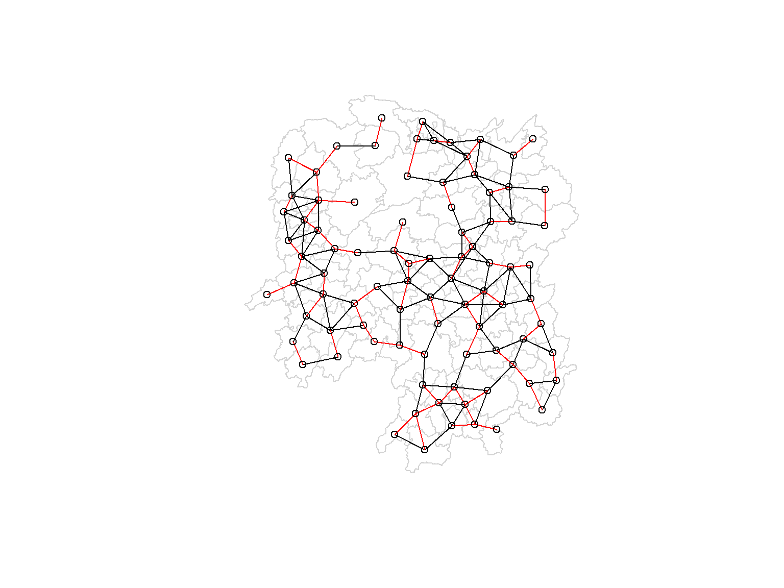
The red lines show the links of 1st nearest neighbours and the black lines show the links of neighbours within the cut-off distance of 62km.
Alternatively, we can plot both of them next to each other by using the code chunk below.
par(mfrow = c(1,2))
plot(hunan$geometry, border = "lightgrey", main = "1st nearest neighbours")
plot(k1, coords, add = TRUE, col = "red", length = 0.88)
plot(hunan$geometry, border = "lightgrey", main = "Distance link")
plot(wm_d62, coords, add = TRUE, pch = 19, cex = 0.6)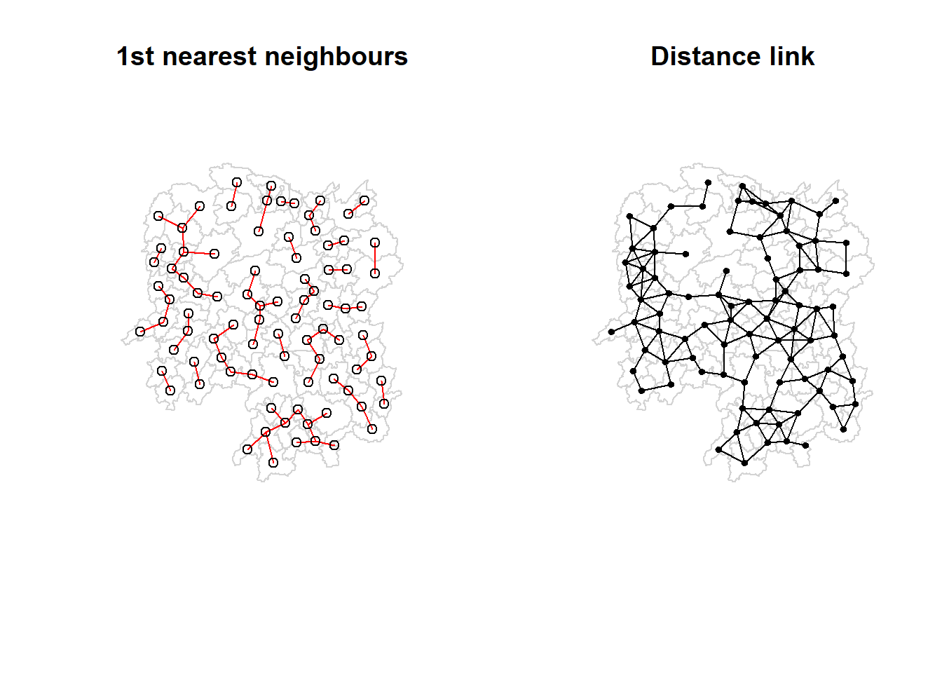
1.6.3 Computing adaptive distance weight matrix
One of the characteristics of fixed distance weight matrix is that the more densely settled areas (usually the urban areas) tend to have more neighbours and the less densely settled areas (usually the rural counties) tend to have lesser neighbours. Having many neighbours soothes the neighbour relationship across more neighbours.
It is possible to control the numbers of neighbours directly using k-nearest neighbours, either accepting asymmetric neighbours or imposing symmetry as shown in the code chunk below.
knn6 <- knn2nb(knearneigh(coords, k=6))
knn6
Neighbour list object:
Number of regions: 88
Number of nonzero links: 528
Percentage nonzero weights: 6.818182
Average number of links: 6
Non-symmetric neighbours listSimilarly, the content of the matrix can be displayed by using str().
str(knn6)List of 88
$ : int [1:6] 2 3 4 5 57 64
$ : int [1:6] 1 3 57 58 78 85
$ : int [1:6] 1 2 4 5 57 85
$ : int [1:6] 1 3 5 6 69 85
$ : int [1:6] 1 3 4 6 69 85
$ : int [1:6] 3 4 5 69 75 85
$ : int [1:6] 9 66 67 71 74 84
$ : int [1:6] 9 46 47 78 80 86
$ : int [1:6] 8 46 66 68 84 86
$ : int [1:6] 16 19 22 70 72 73
$ : int [1:6] 10 14 16 17 70 72
$ : int [1:6] 13 15 60 61 63 83
$ : int [1:6] 12 15 60 61 63 83
$ : int [1:6] 11 15 16 17 72 83
$ : int [1:6] 12 13 14 17 60 83
$ : int [1:6] 10 11 17 22 72 83
$ : int [1:6] 10 11 14 16 72 83
$ : int [1:6] 20 22 23 63 77 83
$ : int [1:6] 10 20 21 73 74 82
$ : int [1:6] 18 19 21 22 23 82
$ : int [1:6] 19 20 35 74 82 86
$ : int [1:6] 10 16 18 19 20 83
$ : int [1:6] 18 20 41 77 79 82
$ : int [1:6] 25 28 31 52 54 81
$ : int [1:6] 24 28 31 33 54 81
$ : int [1:6] 25 27 29 33 42 81
$ : int [1:6] 26 29 30 37 42 81
$ : int [1:6] 24 25 33 49 52 54
$ : int [1:6] 26 27 37 42 43 81
$ : int [1:6] 26 27 28 33 49 81
$ : int [1:6] 24 25 36 39 40 54
$ : int [1:6] 24 31 50 54 55 56
$ : int [1:6] 25 26 28 30 49 81
$ : int [1:6] 36 40 41 45 56 80
$ : int [1:6] 21 41 46 47 80 82
$ : int [1:6] 31 34 40 45 56 80
$ : int [1:6] 26 27 29 42 43 44
$ : int [1:6] 23 43 44 62 77 79
$ : int [1:6] 25 40 42 43 44 81
$ : int [1:6] 31 36 39 43 45 79
$ : int [1:6] 23 35 45 79 80 82
$ : int [1:6] 26 27 37 39 43 81
$ : int [1:6] 37 39 40 42 44 79
$ : int [1:6] 37 38 39 42 43 79
$ : int [1:6] 34 36 40 41 79 80
$ : int [1:6] 8 9 35 47 78 86
$ : int [1:6] 8 21 35 46 80 86
$ : int [1:6] 49 50 51 52 53 55
$ : int [1:6] 28 33 48 51 52 54
$ : int [1:6] 32 48 51 52 54 55
$ : int [1:6] 28 48 49 50 52 54
$ : int [1:6] 28 48 49 50 51 54
$ : int [1:6] 48 50 51 52 55 75
$ : int [1:6] 24 28 49 50 51 52
$ : int [1:6] 32 48 50 52 53 75
$ : int [1:6] 32 34 36 78 80 85
$ : int [1:6] 1 2 3 58 64 68
$ : int [1:6] 2 57 64 66 68 78
$ : int [1:6] 12 13 60 61 87 88
$ : int [1:6] 12 13 59 61 63 87
$ : int [1:6] 12 13 60 62 63 87
$ : int [1:6] 12 38 61 63 77 87
$ : int [1:6] 12 18 60 61 62 83
$ : int [1:6] 1 3 57 58 68 76
$ : int [1:6] 58 64 66 67 68 76
$ : int [1:6] 9 58 67 68 76 84
$ : int [1:6] 7 65 66 68 76 84
$ : int [1:6] 9 57 58 66 78 84
$ : int [1:6] 4 5 6 32 75 85
$ : int [1:6] 10 16 19 22 72 73
$ : int [1:6] 7 19 73 74 84 86
$ : int [1:6] 10 11 14 16 17 70
$ : int [1:6] 10 19 21 70 71 74
$ : int [1:6] 19 21 71 73 84 86
$ : int [1:6] 6 32 50 53 55 69
$ : int [1:6] 58 64 65 66 67 68
$ : int [1:6] 18 23 38 61 62 63
$ : int [1:6] 2 8 9 46 58 68
$ : int [1:6] 38 40 41 43 44 45
$ : int [1:6] 34 35 36 41 45 47
$ : int [1:6] 25 26 28 33 39 42
$ : int [1:6] 19 20 21 23 35 41
$ : int [1:6] 12 13 15 16 22 63
$ : int [1:6] 7 9 66 68 71 74
$ : int [1:6] 2 3 4 5 56 69
$ : int [1:6] 8 9 21 46 47 74
$ : int [1:6] 59 60 61 62 63 88
$ : int [1:6] 59 60 61 62 63 87
- attr(*, "region.id")= chr [1:88] "1" "2" "3" "4" ...
- attr(*, "call")= language knearneigh(x = coords, k = 6)
- attr(*, "sym")= logi FALSE
- attr(*, "type")= chr "knn"
- attr(*, "knn-k")= num 6
- attr(*, "class")= chr "nb"
Note
Notice that each county has six neighbours, no less no more!
1.6.3.1 Plotting distance based neighbours
We can plot the weight matrix using the code chunk below.
plot(hunan$geometry, border = "lightgrey")
plot(knn6, coords, pch = 19, cex = 0.6, add = TRUE, col = "red")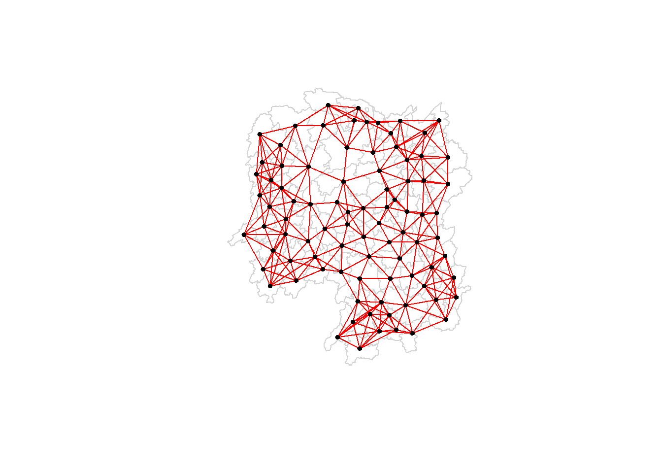
1.7 Weights based on IDW
This section will show how to derive a spatial weight matrix based on Inverse Distance method. Firstly, to compute the distances between areas by using nbdists() of spdep
dist <- nbdists(wm_q, coords, longlat = TRUE)
ids <- lapply(dist, function(x) 1/(x))
ids
[[1]]
[1] 0.01535405 0.03916350 0.01820896 0.02807922 0.01145113
[[2]]
[1] 0.01535405 0.01764308 0.01925924 0.02323898 0.01719350
[[3]]
[1] 0.03916350 0.02822040 0.03695795 0.01395765
[[4]]
[1] 0.01820896 0.02822040 0.03414741 0.01539065
[[5]]
[1] 0.03695795 0.03414741 0.01524598 0.01618354
[[6]]
[1] 0.015390649 0.015245977 0.021748129 0.011883901 0.009810297
[[7]]
[1] 0.01708612 0.01473997 0.01150924 0.01872915
[[8]]
[1] 0.02022144 0.03453056 0.02529256 0.01036340 0.02284457 0.01500600 0.01515314
[[9]]
[1] 0.02022144 0.01574888 0.02109502 0.01508028 0.02902705 0.01502980
[[10]]
[1] 0.02281552 0.01387777 0.01538326 0.01346650 0.02100510 0.02631658 0.01874863
[8] 0.01500046
[[11]]
[1] 0.01882869 0.02243492 0.02247473
[[12]]
[1] 0.02779227 0.02419652 0.02333385 0.02986130 0.02335429
[[13]]
[1] 0.02779227 0.02650020 0.02670323 0.01714243
[[14]]
[1] 0.01882869 0.01233868 0.02098555
[[15]]
[1] 0.02650020 0.01233868 0.01096284 0.01562226
[[16]]
[1] 0.02281552 0.02466962 0.02765018 0.01476814 0.01671430
[[17]]
[1] 0.01387777 0.02243492 0.02098555 0.01096284 0.02466962 0.01593341 0.01437996
[[18]]
[1] 0.02039779 0.02032767 0.01481665 0.01473691 0.01459380
[[19]]
[1] 0.01538326 0.01926323 0.02668415 0.02140253 0.01613589 0.01412874
[[20]]
[1] 0.01346650 0.02039779 0.01926323 0.01723025 0.02153130 0.01469240 0.02327034
[[21]]
[1] 0.02668415 0.01723025 0.01766299 0.02644986 0.02163800
[[22]]
[1] 0.02100510 0.02765018 0.02032767 0.02153130 0.01489296
[[23]]
[1] 0.01481665 0.01469240 0.01401432 0.02246233 0.01880425 0.01530458 0.01849605
[[24]]
[1] 0.02354598 0.01837201 0.02607264 0.01220154 0.02514180
[[25]]
[1] 0.02354598 0.02188032 0.01577283 0.01949232 0.02947957
[[26]]
[1] 0.02155798 0.01745522 0.02212108 0.02220532
[[27]]
[1] 0.02155798 0.02490625 0.01562326
[[28]]
[1] 0.01837201 0.02188032 0.02229549 0.03076171 0.02039506
[[29]]
[1] 0.02490625 0.01686587 0.01395022
[[30]]
[1] 0.02090587
[[31]]
[1] 0.02607264 0.01577283 0.01219005 0.01724850 0.01229012 0.01609781 0.01139438
[8] 0.01150130
[[32]]
[1] 0.01220154 0.01219005 0.01712515 0.01340413 0.01280928 0.01198216 0.01053374
[8] 0.01065655
[[33]]
[1] 0.01949232 0.01745522 0.02229549 0.02090587 0.01979045
[[34]]
[1] 0.03113041 0.03589551 0.02882915
[[35]]
[1] 0.01766299 0.02185795 0.02616766 0.02111721 0.02108253 0.01509020
[[36]]
[1] 0.01724850 0.03113041 0.01571707 0.01860991 0.02073549 0.01680129
[[37]]
[1] 0.01686587 0.02234793 0.01510990 0.01550676
[[38]]
[1] 0.01401432 0.02407426 0.02276151 0.01719415
[[39]]
[1] 0.01229012 0.02172543 0.01711924 0.02629732 0.01896385
[[40]]
[1] 0.01609781 0.01571707 0.02172543 0.01506473 0.01987922 0.01894207
[[41]]
[1] 0.02246233 0.02185795 0.02205991 0.01912542 0.01601083 0.01742892
[[42]]
[1] 0.02212108 0.01562326 0.01395022 0.02234793 0.01711924 0.01836831 0.01683518
[[43]]
[1] 0.01510990 0.02629732 0.01506473 0.01836831 0.03112027 0.01530782
[[44]]
[1] 0.01550676 0.02407426 0.03112027 0.01486508
[[45]]
[1] 0.03589551 0.01860991 0.01987922 0.02205991 0.02107101 0.01982700
[[46]]
[1] 0.03453056 0.04033752 0.02689769
[[47]]
[1] 0.02529256 0.02616766 0.04033752 0.01949145 0.02181458
[[48]]
[1] 0.02313819 0.03370576 0.02289485 0.01630057 0.01818085
[[49]]
[1] 0.03076171 0.02138091 0.02394529 0.01990000
[[50]]
[1] 0.01712515 0.02313819 0.02551427 0.02051530 0.02187179
[[51]]
[1] 0.03370576 0.02138091 0.02873854
[[52]]
[1] 0.02289485 0.02394529 0.02551427 0.02873854 0.03516672
[[53]]
[1] 0.01630057 0.01979945 0.01253977
[[54]]
[1] 0.02514180 0.02039506 0.01340413 0.01990000 0.02051530 0.03516672
[[55]]
[1] 0.01280928 0.01818085 0.02187179 0.01979945 0.01882298
[[56]]
[1] 0.01036340 0.01139438 0.01198216 0.02073549 0.01214479 0.01362855 0.01341697
[[57]]
[1] 0.028079221 0.017643082 0.031423501 0.029114131 0.013520292 0.009903702
[[58]]
[1] 0.01925924 0.03142350 0.02722997 0.01434859 0.01567192
[[59]]
[1] 0.01696711 0.01265572 0.01667105 0.01785036
[[60]]
[1] 0.02419652 0.02670323 0.01696711 0.02343040
[[61]]
[1] 0.02333385 0.01265572 0.02343040 0.02514093 0.02790764 0.01219751 0.02362452
[[62]]
[1] 0.02514093 0.02002219 0.02110260
[[63]]
[1] 0.02986130 0.02790764 0.01407043 0.01805987
[[64]]
[1] 0.02911413 0.01689892
[[65]]
[1] 0.02471705
[[66]]
[1] 0.01574888 0.01726461 0.03068853 0.01954805 0.01810569
[[67]]
[1] 0.01708612 0.01726461 0.01349843 0.01361172
[[68]]
[1] 0.02109502 0.02722997 0.03068853 0.01406357 0.01546511
[[69]]
[1] 0.02174813 0.01645838 0.01419926
[[70]]
[1] 0.02631658 0.01963168 0.02278487
[[71]]
[1] 0.01473997 0.01838483 0.03197403
[[72]]
[1] 0.01874863 0.02247473 0.01476814 0.01593341 0.01963168
[[73]]
[1] 0.01500046 0.02140253 0.02278487 0.01838483 0.01652709
[[74]]
[1] 0.01150924 0.01613589 0.03197403 0.01652709 0.01342099 0.02864567
[[75]]
[1] 0.011883901 0.010533736 0.012539774 0.018822977 0.016458383 0.008217581
[[76]]
[1] 0.01352029 0.01434859 0.01689892 0.02471705 0.01954805 0.01349843 0.01406357
[[77]]
[1] 0.014736909 0.018804247 0.022761507 0.012197506 0.020022195 0.014070428
[7] 0.008440896
[[78]]
[1] 0.02323898 0.02284457 0.01508028 0.01214479 0.01567192 0.01546511 0.01140779
[[79]]
[1] 0.01530458 0.01719415 0.01894207 0.01912542 0.01530782 0.01486508 0.02107101
[[80]]
[1] 0.01500600 0.02882915 0.02111721 0.01680129 0.01601083 0.01982700 0.01949145
[8] 0.01362855
[[81]]
[1] 0.02947957 0.02220532 0.01150130 0.01979045 0.01896385 0.01683518
[[82]]
[1] 0.02327034 0.02644986 0.01849605 0.02108253 0.01742892
[[83]]
[1] 0.023354289 0.017142433 0.015622258 0.016714303 0.014379961 0.014593799
[7] 0.014892965 0.018059871 0.008440896
[[84]]
[1] 0.01872915 0.02902705 0.01810569 0.01361172 0.01342099 0.01297994
[[85]]
[1] 0.011451133 0.017193502 0.013957649 0.016183544 0.009810297 0.010656545
[7] 0.013416965 0.009903702 0.014199260 0.008217581 0.011407794
[[86]]
[1] 0.01515314 0.01502980 0.01412874 0.02163800 0.01509020 0.02689769 0.02181458
[8] 0.02864567 0.01297994
[[87]]
[1] 0.01667105 0.02362452 0.02110260 0.02058034
[[88]]
[1] 0.01785036 0.020580341.8 Row-standardised Weights Matrix
Next, we need to assign weights to each neighbouring polygon. In our case, each neighbouring polygon will be assigned equal weight (style=“W”). This is accomplished by assigning the fraction 1/(#ofneighbours) to each neighbouring county then summing the weighted income values.
While this is the most intuitive way to summaries the neighbours’ values it has one drawback in that polygons along the edges of the study area will base their lagged values on fewer polygons thus potentially over- or under-estimating the true nature of the spatial autocorrelation in the data. For this example, we’ll stick with the style=“W” option for simplicity’s sake but note that other more robust options are available, notably style=“B”.
rswm_q <- nb2listw(wm_q, style = "W", zero.policy = TRUE)
rswm_q
Characteristics of weights list object:
Neighbour list object:
Number of regions: 88
Number of nonzero links: 448
Percentage nonzero weights: 5.785124
Average number of links: 5.090909
Weights style: W
Weights constants summary:
n nn S0 S1 S2
W 88 7744 88 37.86334 365.9147The zero.policy = TRUE option allows for lists of non-neighbours. This should be used with caution since the user may not be aware of missing neighbours in their dataset however, a zero.policy of FALSE would return an error.
To see the weight of the first polygon’s eight neighbours type:
rswm_q$weights[10][[1]]
[1] 0.125 0.125 0.125 0.125 0.125 0.125 0.125 0.125Each neighbour is assigned a value 0.125 of the total weight. This means that when R computes the average neighbouring income values, each neighbour’s income will be multiplied by 0.125 before being tallied.
Using the same method, we can also derive a row standardised distance weight matrix by using the code chunk below.
rswm_ids <- nb2listw(wm_q, glist = ids, style = "B", zero.policy = TRUE)
rswm_ids
Characteristics of weights list object:
Neighbour list object:
Number of regions: 88
Number of nonzero links: 448
Percentage nonzero weights: 5.785124
Average number of links: 5.090909
Weights style: B
Weights constants summary:
n nn S0 S1 S2
B 88 7744 8.786867 0.3776535 3.8137rswm_ids$weights[1][[1]]
[1] 0.01535405 0.03916350 0.01820896 0.02807922 0.01145113Results of previous code chunk shown above.
summary(unlist(rswm_ids$weights)) Min. 1st Qu. Median Mean 3rd Qu. Max.
0.008218 0.015088 0.018739 0.019614 0.022823 0.040338 1.9 Application of Spatial Weight Matrix
In this section, it shows how to create four different spatial lagged variables, they are:
- spatial lag with row-standardized weights,
- spatial lag as a sum of neighbouring values,
- spatial window average, and
- spatial window sum.
1.9.1 Spatial lag with row-standardized weights
Finally, we’ll compute the average neighbour GDPPC value for each polygon. These values are often referred to as spatially lagged values.
GDPPC.lag <- lag.listw(rswm_q, hunan$GDPPC)
GDPPC.lag
[1] 24847.20 22724.80 24143.25 27737.50 27270.25 21248.80 43747.00 33582.71
[9] 45651.17 32027.62 32671.00 20810.00 25711.50 30672.33 33457.75 31689.20
[17] 20269.00 23901.60 25126.17 21903.43 22718.60 25918.80 20307.00 20023.80
[25] 16576.80 18667.00 14394.67 19848.80 15516.33 20518.00 17572.00 15200.12
[33] 18413.80 14419.33 24094.50 22019.83 12923.50 14756.00 13869.80 12296.67
[41] 15775.17 14382.86 11566.33 13199.50 23412.00 39541.00 36186.60 16559.60
[49] 20772.50 19471.20 19827.33 15466.80 12925.67 18577.17 14943.00 24913.00
[57] 25093.00 24428.80 17003.00 21143.75 20435.00 17131.33 24569.75 23835.50
[65] 26360.00 47383.40 55157.75 37058.00 21546.67 23348.67 42323.67 28938.60
[73] 25880.80 47345.67 18711.33 29087.29 20748.29 35933.71 15439.71 29787.50
[81] 18145.00 21617.00 29203.89 41363.67 22259.09 44939.56 16902.00 16930.00Recall in the previous section, we retrieved the GDPPC of these five countries by using the code chunk below:
nb1 <- wm_q[[1]]
nb1 <- hunan$GDPPC[nb1]
nb1
[1] 20981 34592 24473 21311 22879We can append the spatially lag GDPPC values onto hunan sf data frame by using the code chunk below.
lag.list <- list(hunan$NAME_3, lag.listw(rswm_q, hunan$GDPPC))
lag.res <- as.data.frame(lag.list)
colnames(lag.res) <- c("NAME_3", "lag GDPPC")
hunan <- left_join(hunan,lag.res)
Joining with `by = join_by(NAME_3)`The following table shows the average neighboring income values (stored in the Inc.lag object) for each county.
head(hunan)Simple feature collection with 6 features and 7 fields
Geometry type: POLYGON
Dimension: XY
Bounding box: xmin: 110.4922 ymin: 28.61762 xmax: 112.3013 ymax: 30.12812
Geodetic CRS: WGS 84
NAME_2 ID_3 NAME_3 ENGTYPE_3 County GDPPC lag GDPPC
1 Changde 21098 Anxiang County Anxiang 23667 24847.20
2 Changde 21100 Hanshou County Hanshou 20981 22724.80
3 Changde 21101 Jinshi County City Jinshi 34592 24143.25
4 Changde 21102 Li County Li 24473 27737.50
5 Changde 21103 Linli County Linli 25554 27270.25
6 Changde 21104 Shimen County Shimen 27137 21248.80
geometry
1 POLYGON ((112.0625 29.75523...
2 POLYGON ((112.2288 29.11684...
3 POLYGON ((111.8927 29.6013,...
4 POLYGON ((111.3731 29.94649...
5 POLYGON ((111.6324 29.76288...
6 POLYGON ((110.8825 30.11675...Next, to plot both the GDPPC and spatial lag GDPPC for comparison using the code chunk below.
gdppc <- qtm(hunan, "GDPPC")
lag_gdppc <- qtm(hunan, "lag GDPPC")
tmap_arrange(gdppc, lag_gdppc, asp = 1, ncol = 2)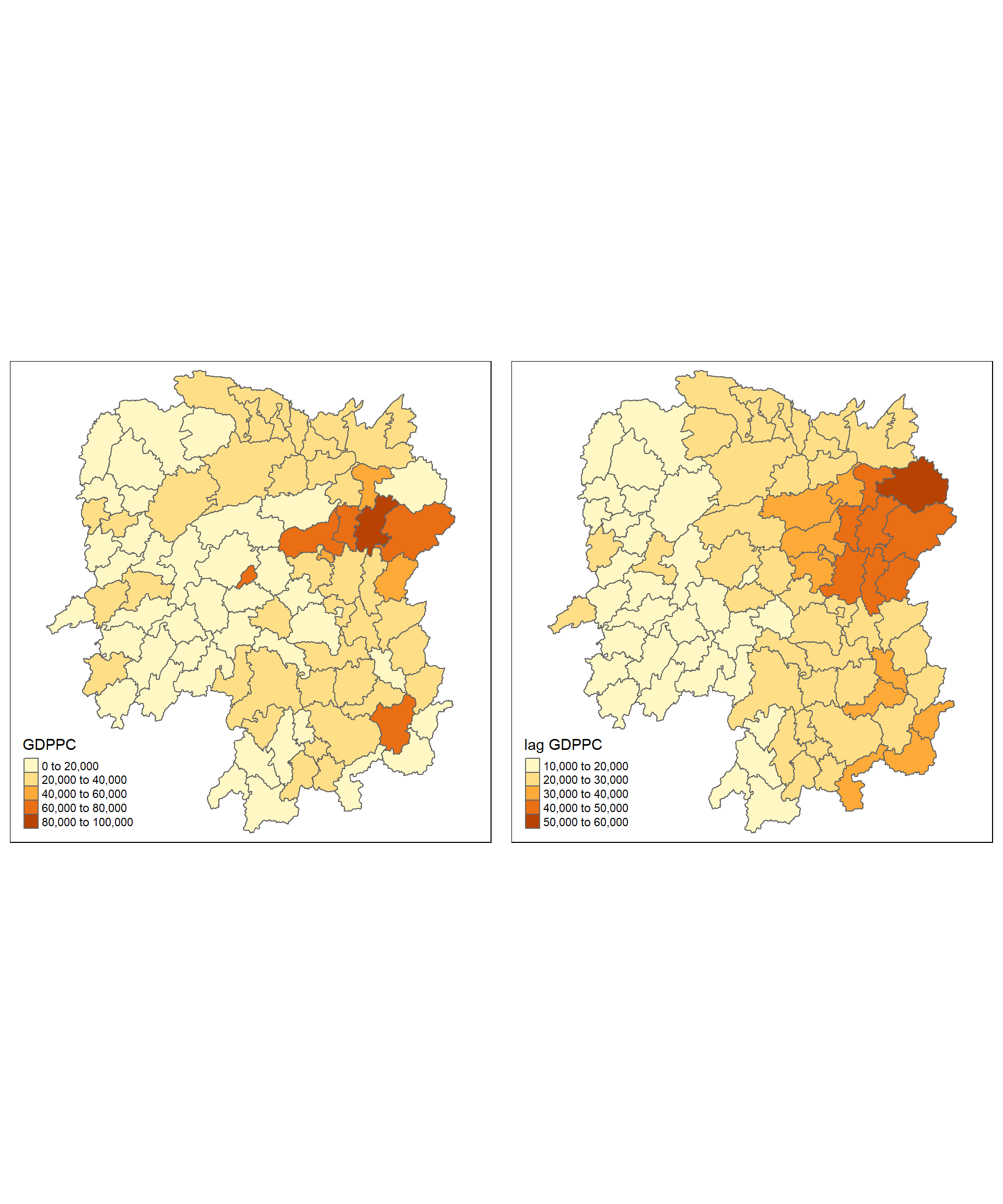
1.9.2 Spatial lag as a sum of neighboring values
We can calculate spatial lag as a sum of neighbouring values by assigning binary weights. This requires us to go back to our neighbours list, then apply a function that will assign binary weights, then we use glist = in the nb2listw function to explicitly assign these weights.
We start by applying a function that will assign a value of 1 per each neighbour. This is done with lapply(), which we have been using to manipulate the neighbours structure throughout the past notebooks. Basically it applies a function across each value in the neighbours structure.
b_weights <- lapply(wm_q, function(x) 0*x + 1)
b_weights2 <- nb2listw(wm_q,
                       glist = b_weights,
                       style = "B")
b_weights2
Characteristics of weights list object:
Neighbour list object:
Number of regions: 88
Number of nonzero links: 448
Percentage nonzero weights: 5.785124
Average number of links: 5.090909
Weights style: B
Weights constants summary:
n nn S0 S1 S2
B 88 7744 448 896 10224With the proper weights assigned, we can use lag.listw() to compute a lag variable from our weight and GDPPC.
lag_sum <- list(hunan$NAME_3, lag.listw(b_weights2, hunan$GDPPC))
lag.res <- as.data.frame(lag_sum)
colnames(lag.res) <- c("NAME_3", "lag_sum GDPPC")
First, to examine the result by using the code chunk below.
lag_sum[[1]]
[1] "Anxiang" "Hanshou" "Jinshi" "Li"
[5] "Linli" "Shimen" "Liuyang" "Ningxiang"
[9] "Wangcheng" "Anren" "Guidong" "Jiahe"
[13] "Linwu" "Rucheng" "Yizhang" "Yongxing"
[17] "Zixing" "Changning" "Hengdong" "Hengnan"
[21] "Hengshan" "Leiyang" "Qidong" "Chenxi"
[25] "Zhongfang" "Huitong" "Jingzhou" "Mayang"
[29] "Tongdao" "Xinhuang" "Xupu" "Yuanling"
[33] "Zhijiang" "Lengshuijiang" "Shuangfeng" "Xinhua"
[37] "Chengbu" "Dongan" "Dongkou" "Longhui"
[41] "Shaodong" "Suining" "Wugang" "Xinning"
[45] "Xinshao" "Shaoshan" "Xiangxiang" "Baojing"
[49] "Fenghuang" "Guzhang" "Huayuan" "Jishou"
[53] "Longshan" "Luxi" "Yongshun" "Anhua"
[57] "Nan" "Yuanjiang" "Jianghua" "Lanshan"
[61] "Ningyuan" "Shuangpai" "Xintian" "Huarong"
[65] "Linxiang" "Miluo" "Pingjiang" "Xiangyin"
[69] "Cili" "Chaling" "Liling" "Yanling"
[73] "You" "Zhuzhou" "Sangzhi" "Yueyang"
[77] "Qiyang" "Taojiang" "Shaoyang" "Lianyuan"
[81] "Hongjiang" "Hengyang" "Guiyang" "Changsha"
[85] "Taoyuan" "Xiangtan" "Dao" "Jiangyong"
[[2]]
[1] 124236 113624 96573 110950 109081 106244 174988 235079 273907 256221
[11] 98013 104050 102846 92017 133831 158446 141883 119508 150757 153324
[21] 113593 129594 142149 100119 82884 74668 43184 99244 46549 20518
[31] 140576 121601 92069 43258 144567 132119 51694 59024 69349 73780
[41] 94651 100680 69398 52798 140472 118623 180933 82798 83090 97356
[51] 59482 77334 38777 111463 74715 174391 150558 122144 68012 84575
[61] 143045 51394 98279 47671 26360 236917 220631 185290 64640 70046
[71] 126971 144693 129404 284074 112268 203611 145238 251536 108078 238300
[81] 108870 108085 262835 248182 244850 404456 67608 33860Next, to append the lag_sum GDPPC field into hunan sf data frame by using the code chunk below.
hunan <- left_join(hunan, lag.res)Joining with `by = join_by(NAME_3)`Following which, to plot both the GDPPC and Spatial Lag Sum GDPPC for comparison using the code chunk below.
gdppc <- qtm(hunan, "GDPPC")
lag_sum_gdppc <- qtm(hunan, "lag_sum GDPPC")
tmap_arrange(gdppc, lag_sum_gdppc, asp = 1, ncol = 2)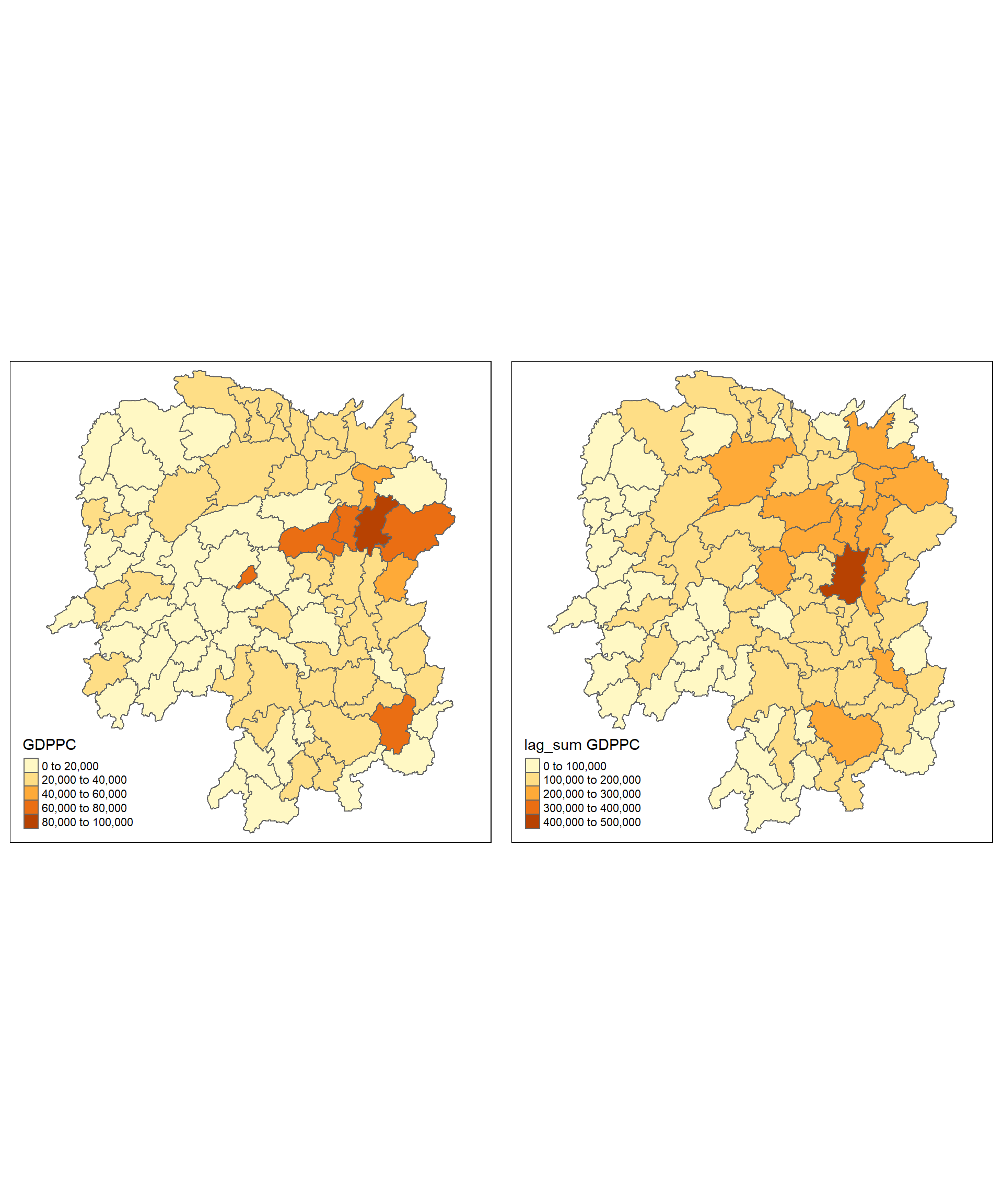
1.9.3 Spatial window average
The spatial window average uses row-standardized weights and includes the diagonal element. To do this in R, we need to go back to the neighbors structure and add the diagonal element before assigning weights.
To add the diagonal element to the neighbour list, we just need to use include.self() from spdep.
wm_qs <- include.self(wm_q)Notice that the Number of non-zero links, Percentage non-zero weights and Average number of links are 536, 6.921488 and 6.090909 respectively as compared to wm_q of 448, 5.785124 and 5.090909
Let us take a good look at the neighbour list of area [1] by using the code chunk below.
wm_qs[[1]][1] 1 2 3 4 57 85Notice that now [1] has six neighbours instead of five.
Now we obtain weights with nb2listw()
wm_qs <- nb2listw(wm_qs)
wm_qs
Characteristics of weights list object:
Neighbour list object:
Number of regions: 88
Number of nonzero links: 536
Percentage nonzero weights: 6.921488
Average number of links: 6.090909
Weights style: W
Weights constants summary:
n nn S0 S1 S2
W 88 7744 88 30.90265 357.5308Again, utilising nb2listw() and glist() to explicitly assign weight values.
Lastly, we just need to create the lag variable from our weight structure and GDPPC variable.
lag_w_avg_gpdpc <- lag.listw(wm_qs,
                             hunan$GDPPC)
lag_w_avg_gpdpc
[1] 24650.50 22434.17 26233.00 27084.60 26927.00 22230.17 47621.20 37160.12
[9] 49224.71 29886.89 26627.50 22690.17 25366.40 25825.75 30329.00 32682.83
[17] 25948.62 23987.67 25463.14 21904.38 23127.50 25949.83 20018.75 19524.17
[25] 18955.00 17800.40 15883.00 18831.33 14832.50 17965.00 17159.89 16199.44
[33] 18764.50 26878.75 23188.86 20788.14 12365.20 15985.00 13764.83 11907.43
[41] 17128.14 14593.62 11644.29 12706.00 21712.29 43548.25 35049.00 16226.83
[49] 19294.40 18156.00 19954.75 18145.17 12132.75 18419.29 14050.83 23619.75
[57] 24552.71 24733.67 16762.60 20932.60 19467.75 18334.00 22541.00 26028.00
[65] 29128.50 46569.00 47576.60 36545.50 20838.50 22531.00 42115.50 27619.00
[73] 27611.33 44523.29 18127.43 28746.38 20734.50 33880.62 14716.38 28516.22
[81] 18086.14 21244.50 29568.80 48119.71 22310.75 43151.60 17133.40 17009.33Next, to convert the lag variable listw object into a data.frame by using as.data.frame().
lag.list.wm_qs <- list(hunan$NAME_3, lag.listw(wm_qs, hunan$GDPPC))
lag_wm_qs.res <- as.data.frame(lag.list.wm_qs)
colnames(lag_wm_qs.res) <- c("NAME_3", "lag_window_avg GDPPC")
Note
The third command line on the code chunk above renames the field names of lag_wm_q1.res object into NAME_3 and lag_window_avg GDPPC respectively.
Next, the code chunk below will be used to append lag_window_avg GDPPC values onto hunan sf data.frame by using left_join() of dplyr package.
hunan <- left_join(hunan, lag_wm_qs.res)Joining with `by = join_by(NAME_3)`To compare the values of lag GDPPC and Spatial window average, kable() of Knitr package is used to prepare a table using the code chunk below.
hunan %>%
  select("County",
         "lag GDPPC",
         "lag_window_avg GDPPC") %>%
kable()| County | lag GDPPC | lag_window_avg GDPPC | geometry |
|---|---|---|---|
| Anxiang | 24847.20 | 24650.50 | POLYGON ((112.0625 29.75523… |
| Hanshou | 22724.80 | 22434.17 | POLYGON ((112.2288 29.11684… |
| Jinshi | 24143.25 | 26233.00 | POLYGON ((111.8927 29.6013,… |
| Li | 27737.50 | 27084.60 | POLYGON ((111.3731 29.94649… |
| Linli | 27270.25 | 26927.00 | POLYGON ((111.6324 29.76288… |
| Shimen | 21248.80 | 22230.17 | POLYGON ((110.8825 30.11675… |
| Liuyang | 43747.00 | 47621.20 | POLYGON ((113.9905 28.5682,… |
| Ningxiang | 33582.71 | 37160.12 | POLYGON ((112.7181 28.38299… |
| Wangcheng | 45651.17 | 49224.71 | POLYGON ((112.7914 28.52688… |
| Anren | 32027.62 | 29886.89 | POLYGON ((113.1757 26.82734… |
| Guidong | 32671.00 | 26627.50 | POLYGON ((114.1799 26.20117… |
| Jiahe | 20810.00 | 22690.17 | POLYGON ((112.4425 25.74358… |
| Linwu | 25711.50 | 25366.40 | POLYGON ((112.5914 25.55143… |
| Rucheng | 30672.33 | 25825.75 | POLYGON ((113.6759 25.87578… |
| Yizhang | 33457.75 | 30329.00 | POLYGON ((113.2621 25.68394… |
| Yongxing | 31689.20 | 32682.83 | POLYGON ((113.3169 26.41843… |
| Zixing | 20269.00 | 25948.62 | POLYGON ((113.7311 26.16259… |
| Changning | 23901.60 | 23987.67 | POLYGON ((112.6144 26.60198… |
| Hengdong | 25126.17 | 25463.14 | POLYGON ((113.1056 27.21007… |
| Hengnan | 21903.43 | 21904.38 | POLYGON ((112.7599 26.98149… |
| Hengshan | 22718.60 | 23127.50 | POLYGON ((112.607 27.4689, … |
| Leiyang | 25918.80 | 25949.83 | POLYGON ((112.9996 26.69276… |
| Qidong | 20307.00 | 20018.75 | POLYGON ((111.7818 27.0383,… |
| Chenxi | 20023.80 | 19524.17 | POLYGON ((110.2624 28.21778… |
| Zhongfang | 16576.80 | 18955.00 | POLYGON ((109.9431 27.72858… |
| Huitong | 18667.00 | 17800.40 | POLYGON ((109.9419 27.10512… |
| Jingzhou | 14394.67 | 15883.00 | POLYGON ((109.8186 26.75842… |
| Mayang | 19848.80 | 18831.33 | POLYGON ((109.795 27.98008,… |
| Tongdao | 15516.33 | 14832.50 | POLYGON ((109.9294 26.46561… |
| Xinhuang | 20518.00 | 17965.00 | POLYGON ((109.227 27.43733,… |
| Xupu | 17572.00 | 17159.89 | POLYGON ((110.7189 28.30485… |
| Yuanling | 15200.12 | 16199.44 | POLYGON ((110.9652 28.99895… |
| Zhijiang | 18413.80 | 18764.50 | POLYGON ((109.8818 27.60661… |
| Lengshuijiang | 14419.33 | 26878.75 | POLYGON ((111.5307 27.81472… |
| Shuangfeng | 24094.50 | 23188.86 | POLYGON ((112.263 27.70421,… |
| Xinhua | 22019.83 | 20788.14 | POLYGON ((111.3345 28.19642… |
| Chengbu | 12923.50 | 12365.20 | POLYGON ((110.4455 26.69317… |
| Dongan | 14756.00 | 15985.00 | POLYGON ((111.4531 26.86812… |
| Dongkou | 13869.80 | 13764.83 | POLYGON ((110.6622 27.37305… |
| Longhui | 12296.67 | 11907.43 | POLYGON ((110.985 27.65983,… |
| Shaodong | 15775.17 | 17128.14 | POLYGON ((111.9054 27.40254… |
| Suining | 14382.86 | 14593.62 | POLYGON ((110.389 27.10006,… |
| Wugang | 11566.33 | 11644.29 | POLYGON ((110.9878 27.03345… |
| Xinning | 13199.50 | 12706.00 | POLYGON ((111.0736 26.84627… |
| Xinshao | 23412.00 | 21712.29 | POLYGON ((111.6013 27.58275… |
| Shaoshan | 39541.00 | 43548.25 | POLYGON ((112.5391 27.97742… |
| Xiangxiang | 36186.60 | 35049.00 | POLYGON ((112.4549 28.05783… |
| Baojing | 16559.60 | 16226.83 | POLYGON ((109.7015 28.82844… |
| Fenghuang | 20772.50 | 19294.40 | POLYGON ((109.5239 28.19206… |
| Guzhang | 19471.20 | 18156.00 | POLYGON ((109.8968 28.74034… |
| Huayuan | 19827.33 | 19954.75 | POLYGON ((109.5647 28.61712… |
| Jishou | 15466.80 | 18145.17 | POLYGON ((109.8375 28.4696,… |
| Longshan | 12925.67 | 12132.75 | POLYGON ((109.6337 29.62521… |
| Luxi | 18577.17 | 18419.29 | POLYGON ((110.1067 28.41835… |
| Yongshun | 14943.00 | 14050.83 | POLYGON ((110.0003 29.29499… |
| Anhua | 24913.00 | 23619.75 | POLYGON ((111.6034 28.63716… |
| Nan | 25093.00 | 24552.71 | POLYGON ((112.3232 29.46074… |
| Yuanjiang | 24428.80 | 24733.67 | POLYGON ((112.4391 29.1791,… |
| Jianghua | 17003.00 | 16762.60 | POLYGON ((111.6461 25.29661… |
| Lanshan | 21143.75 | 20932.60 | POLYGON ((112.2286 25.61123… |
| Ningyuan | 20435.00 | 19467.75 | POLYGON ((112.0715 26.09892… |
| Shuangpai | 17131.33 | 18334.00 | POLYGON ((111.8864 26.11957… |
| Xintian | 24569.75 | 22541.00 | POLYGON ((112.2578 26.0796,… |
| Huarong | 23835.50 | 26028.00 | POLYGON ((112.9242 29.69134… |
| Linxiang | 26360.00 | 29128.50 | POLYGON ((113.5502 29.67418… |
| Miluo | 47383.40 | 46569.00 | POLYGON ((112.9902 29.02139… |
| Pingjiang | 55157.75 | 47576.60 | POLYGON ((113.8436 29.06152… |
| Xiangyin | 37058.00 | 36545.50 | POLYGON ((112.9173 28.98264… |
| Cili | 21546.67 | 20838.50 | POLYGON ((110.8822 29.69017… |
| Chaling | 23348.67 | 22531.00 | POLYGON ((113.7666 27.10573… |
| Liling | 42323.67 | 42115.50 | POLYGON ((113.5673 27.94346… |
| Yanling | 28938.60 | 27619.00 | POLYGON ((113.9292 26.6154,… |
| You | 25880.80 | 27611.33 | POLYGON ((113.5879 27.41324… |
| Zhuzhou | 47345.67 | 44523.29 | POLYGON ((113.2493 28.02411… |
| Sangzhi | 18711.33 | 18127.43 | POLYGON ((110.556 29.40543,… |
| Yueyang | 29087.29 | 28746.38 | POLYGON ((113.343 29.61064,… |
| Qiyang | 20748.29 | 20734.50 | POLYGON ((111.5563 26.81318… |
| Taojiang | 35933.71 | 33880.62 | POLYGON ((112.0508 28.67265… |
| Shaoyang | 15439.71 | 14716.38 | POLYGON ((111.5013 27.30207… |
| Lianyuan | 29787.50 | 28516.22 | POLYGON ((111.6789 28.02946… |
| Hongjiang | 18145.00 | 18086.14 | POLYGON ((110.1441 27.47513… |
| Hengyang | 21617.00 | 21244.50 | POLYGON ((112.7144 26.98613… |
| Guiyang | 29203.89 | 29568.80 | POLYGON ((113.0811 26.04963… |
| Changsha | 41363.67 | 48119.71 | POLYGON ((112.9421 28.03722… |
| Taoyuan | 22259.09 | 22310.75 | POLYGON ((112.0612 29.32855… |
| Xiangtan | 44939.56 | 43151.60 | POLYGON ((113.0426 27.8942,… |
| Dao | 16902.00 | 17133.40 | POLYGON ((111.498 25.81679,… |
| Jiangyong | 16930.00 | 17009.33 | POLYGON ((111.3659 25.39472… |
Lastly, qtm() of tmap package is used to plot the lag_gdppc and w_ave_gdppc maps next to each other for quick comparison.
w_avg_gdppc <- qtm(hunan, "lag_window_avg GDPPC")
tmap_arrange(lag_gdppc, w_avg_gdppc, asp=1, ncol=2)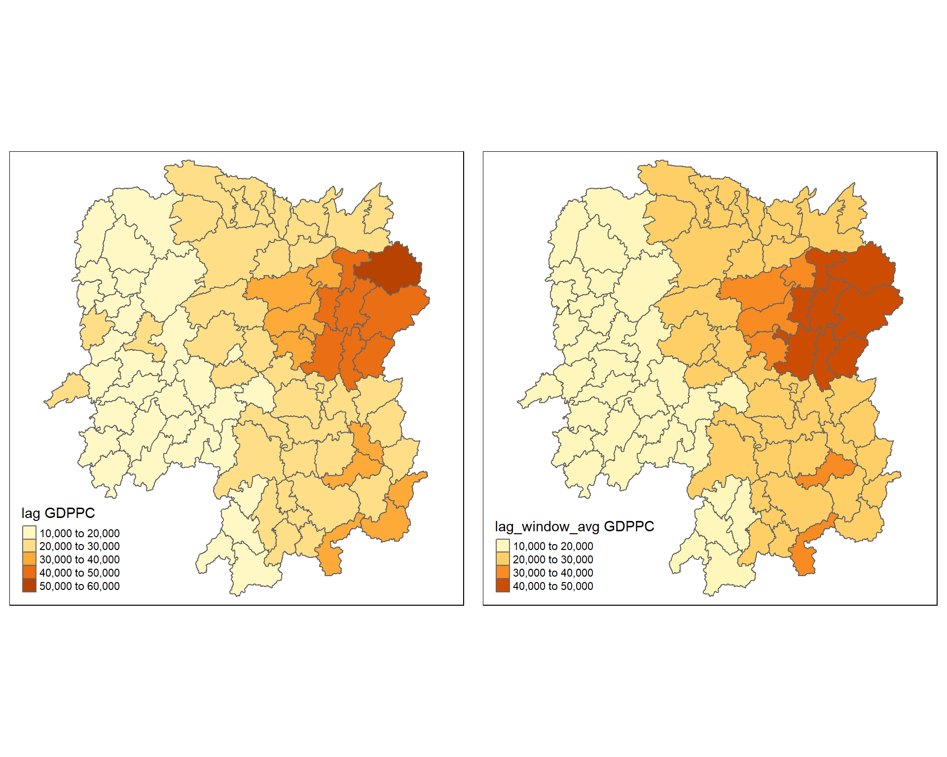
Tip
For more effective comparison, it is advisable to use the core tmap mapping functions.
1.9.4 Spatial window sum
The spatial window sum is the counter part of the window average, but without using row-standardized weights.
To add the diagonal element to the neighbour list, we just need to use include.self() from spdep.
wm_qs <- include.self(wm_q)
wm_qs
Neighbour list object:
Number of regions: 88
Number of nonzero links: 536
Percentage nonzero weights: 6.921488
Average number of links: 6.090909 Assigning binary weights to the neighbour structure that includes the diagonal element.
b_weights <- lapply(wm_qs, function(x) 0*x + 1)
b_weights[1][[1]]
[1] 1 1 1 1 1 1Notice that now [1] has six neighbours instead of five.
Again, we use nb2listw() and glist() to explicitly assign weight values.
b_weights2 <- nb2listw(wm_qs,
glist = b_weights,
style = "B")
b_weights2Characteristics of weights list object:
Neighbour list object:
Number of regions: 88
Number of nonzero links: 536
Percentage nonzero weights: 6.921488
Average number of links: 6.090909
Weights style: B
Weights constants summary:
n nn S0 S1 S2
B 88 7744 536 1072 14160With our new weight structure, we can compute the lag variable with lag.listw().
w_sum_gdppc <- list(hunan$NAME_3, lag.listw(b_weights2, hunan$GDPPC))
w_sum_gdppc
[[1]]
[1] "Anxiang" "Hanshou" "Jinshi" "Li"
[5] "Linli" "Shimen" "Liuyang" "Ningxiang"
[9] "Wangcheng" "Anren" "Guidong" "Jiahe"
[13] "Linwu" "Rucheng" "Yizhang" "Yongxing"
[17] "Zixing" "Changning" "Hengdong" "Hengnan"
[21] "Hengshan" "Leiyang" "Qidong" "Chenxi"
[25] "Zhongfang" "Huitong" "Jingzhou" "Mayang"
[29] "Tongdao" "Xinhuang" "Xupu" "Yuanling"
[33] "Zhijiang" "Lengshuijiang" "Shuangfeng" "Xinhua"
[37] "Chengbu" "Dongan" "Dongkou" "Longhui"
[41] "Shaodong" "Suining" "Wugang" "Xinning"
[45] "Xinshao" "Shaoshan" "Xiangxiang" "Baojing"
[49] "Fenghuang" "Guzhang" "Huayuan" "Jishou"
[53] "Longshan" "Luxi" "Yongshun" "Anhua"
[57] "Nan" "Yuanjiang" "Jianghua" "Lanshan"
[61] "Ningyuan" "Shuangpai" "Xintian" "Huarong"
[65] "Linxiang" "Miluo" "Pingjiang" "Xiangyin"
[69] "Cili" "Chaling" "Liling" "Yanling"
[73] "You" "Zhuzhou" "Sangzhi" "Yueyang"
[77] "Qiyang" "Taojiang" "Shaoyang" "Lianyuan"
[81] "Hongjiang" "Hengyang" "Guiyang" "Changsha"
[85] "Taoyuan" "Xiangtan" "Dao" "Jiangyong"
[[2]]
[1] 147903 134605 131165 135423 134635 133381 238106 297281 344573 268982
[11] 106510 136141 126832 103303 151645 196097 207589 143926 178242 175235
[21] 138765 155699 160150 117145 113730 89002 63532 112988 59330 35930
[31] 154439 145795 112587 107515 162322 145517 61826 79925 82589 83352
[41] 119897 116749 81510 63530 151986 174193 210294 97361 96472 108936
[51] 79819 108871 48531 128935 84305 188958 171869 148402 83813 104663
[61] 155742 73336 112705 78084 58257 279414 237883 219273 83354 90124
[71] 168462 165714 165668 311663 126892 229971 165876 271045 117731 256646
[81] 126603 127467 295688 336838 267729 431516 85667 51028Next, we will convert the lag variable listw object into a data.frame by using as.data.frame().
w_sum_gdppc.res <- as.data.frame(w_sum_gdppc)
colnames(w_sum_gdppc.res) <- c("NAME_3", "w_sum GDPPC")
Note: The second command line on the code chunk above renames the field names of w_sum_gdppc.res object into NAME_3 and w_sum GDPPC respectively.
Next, the code chunk below will be used to append w_sum GDPPC values onto hunan sf data.frame by using left_join() of dplyr package.
hunan <- left_join(hunan, w_sum_gdppc.res)Joining with `by = join_by(NAME_3)`Once again, qtm() of tmap package is used to plot the lag_sum GDPPC and w_sum_gdppc maps next to each other for quick comparison.
w_sum_gdppc <- qtm(hunan, "w_sum GDPPC")
tmap_arrange(lag_sum_gdppc, w_sum_gdppc, asp=1, ncol=2)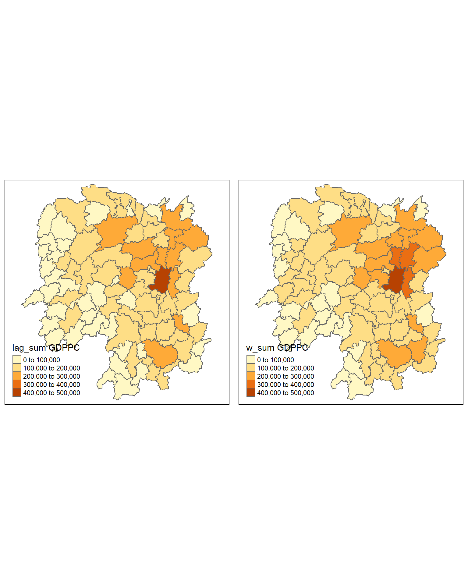
Note
It is advisable to use the core tmap mapping functions for a more effective comparison.