install.packages("maptools",
repos = "https://packagemanager.posit.co/cran/2023-10-13")In-class Exercise 2
2 Spatial Point Pattern Analysis
2.1 Issue 1: Installing maptools
maptools is already retired and binary is removed from CRAN. However, we can download it from Posit Public Package Manager snapshots by using the code chunk below.
However, after installation is completed it is important to note the usage of code chunk below to avoid maptools from being re-downloaded and being installed repetitively every time the Quarto document has been rendered.
2.2 Loading R packages
pacman::p_load(sf, raster, spatstat, tmap, tidyverse)2.3 Issue 2: Creating coastal outline
In sf package, there are two functions that allow us to combine multiple simple features into one simple features. They are st_combine() and st_union().
st_combine()returns a single, combined geometry, with no resolved boundaries; returned geometries may well be invalid.If y is missing,
st_union(x)returns a single geometry with resolved boundaries, else the geometries for all union-ed pairs of x[i] and y[j].
childcare_sf <- st_read("data/child-care-services-geojson.geojson") %>%
  st_transform(crs = 3414)
mpsz_sf <- st_read(dsn = "data", layer="MP14_SUBZONE_WEB_PL")Reading layer `MP14_SUBZONE_WEB_PL' from data source
`C:\zjho008\ISSS626-GAA\In-class_Ex\In-class_Ex02\data' using driver `ESRI Shapefile'
Simple feature collection with 323 features and 15 fields
Geometry type: MULTIPOLYGON
Dimension: XY
Bounding box: xmin: 2667.538 ymin: 15748.72 xmax: 56396.44 ymax: 50256.33
Projected CRS: SVY212.4 Working with st_union()
In code chunk below, st_union() is used to derive the coastal outline sf tibble data.frame
sg_sf <- mpsz_sf %>%
  st_union()
sg_sf will look similar to the figure shown below using the following code chunk:
plot(sg_sf)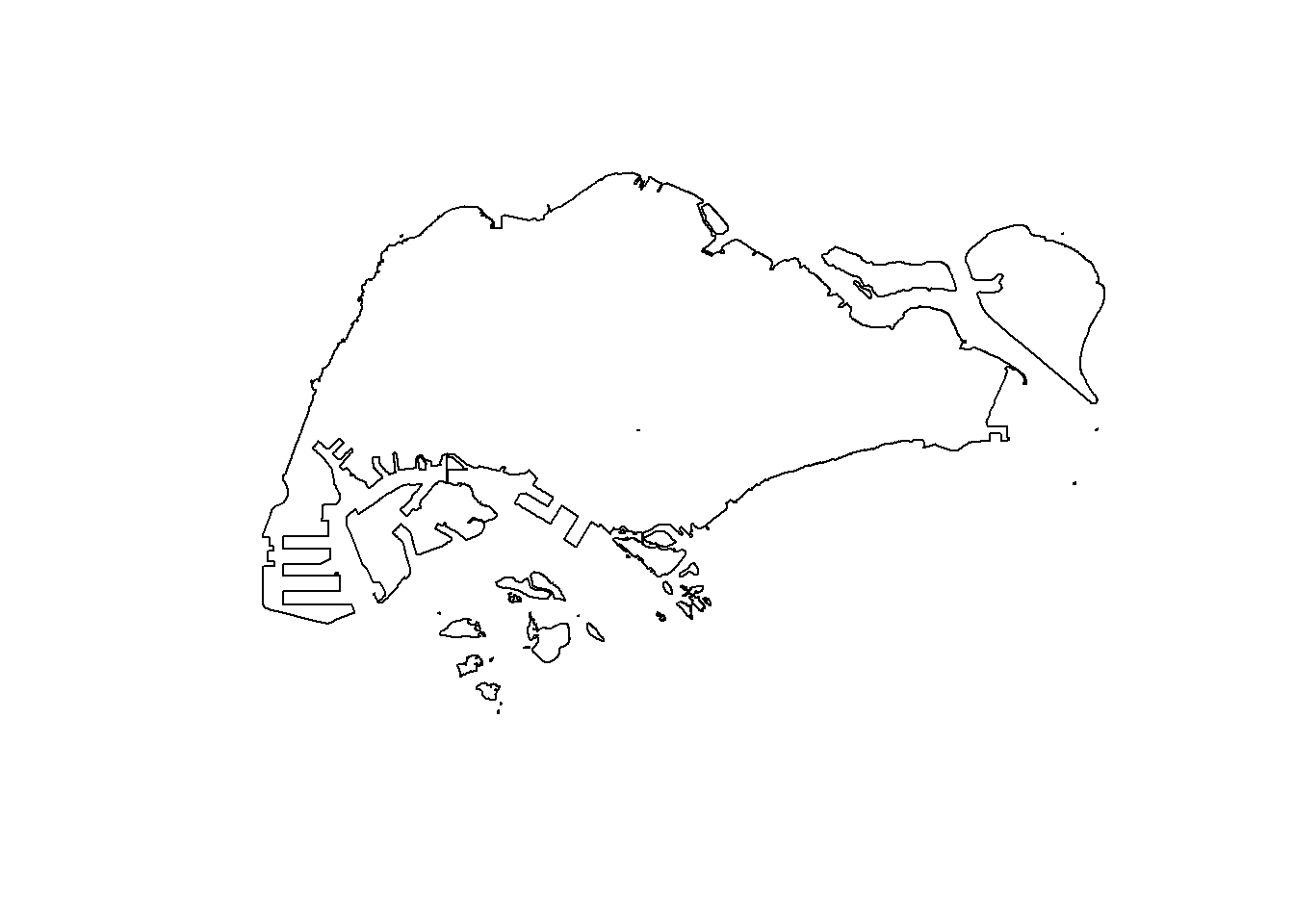
2.5 spatstat package
spatstat R package is a comprehensive open-source toolbox for analysing Spatial Point Patterns. It focuses on two-dimensional point patterns, including multi-type or marked points, in any spatial region.
2.6 spatstat
2.6.1 spatstat sub-packages
- The spatstat package now contains only documentation and introductory material. It provides beginner’s introductions, vignettes, interactive demonstration scripts, and a few help files summarising the package.
- The spatstat.data package now contains all the datasets for spatstat.
- The spatstat.utils package contains basic utility functions for spatstat.
- The spatstat.univar package contains functions for estimating and manipulating probability distributions of one-dimensional random variables.
- The spatstat.sparse package contains functions for manipulating sparse arrays and performing linear algebra.
- The spatstat.geom package contains definitions of spatial objects (such as point patterns, windows and pixel images) and code which performs geometrical operations.
- The spatstat.random package contains functions for random generation of spatial patterns and random simulation of models.
- The spatstat.explore package contains the code for exploratory data analysis and nonparametric analysis of spatial data.
- The spatstat.model package contains the code for model-fitting, model diagnostics, and formal inference.
- The spatstat.linnet package defines spatial data on a linear network, and performs geometrical operations and statistical analysis on such data.
2.7 Creating ppp objects from sf data.frame
Working with sf data.frame
In the code chunk below, as.ppp() of spatstat.geom package is used to derive a ppp object layer directly from a sf tibble data.frame.
childcare_ppp <- as.ppp(childcare_sf)Warning in as.ppp.sf(childcare_sf): only first attribute column is used for
marksplot(childcare_ppp)Warning in default.charmap(ntypes, chars): Too many types to display every type
as a different characterWarning: Only 10 out of 1545 symbols are shown in the symbol map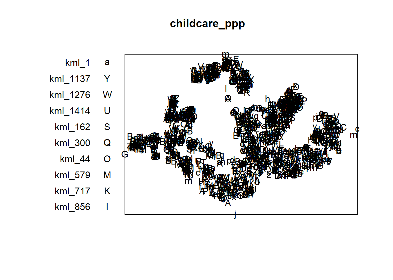
summary() function is used to reveal properties of the ppp object created
summary(childcare_ppp)Marked planar point pattern: 1545 points
Average intensity 1.91145e-06 points per square unit
Coordinates are given to 11 decimal places
marks are of type 'character'
Summary:
Length Class Mode
1545 character character
Window: rectangle = [11203.01, 45404.24] x [25667.6, 49300.88] units
(34200 x 23630 units)
Window area = 808287000 square units2.8 Creating owin object from sf data.frame
The code chunk as.owin() of spatstat.geom is used to create an owin object class from polygon sf tibble data.frame.
sg_owin <- as.owin(sg_sf)
plot(sg_owin)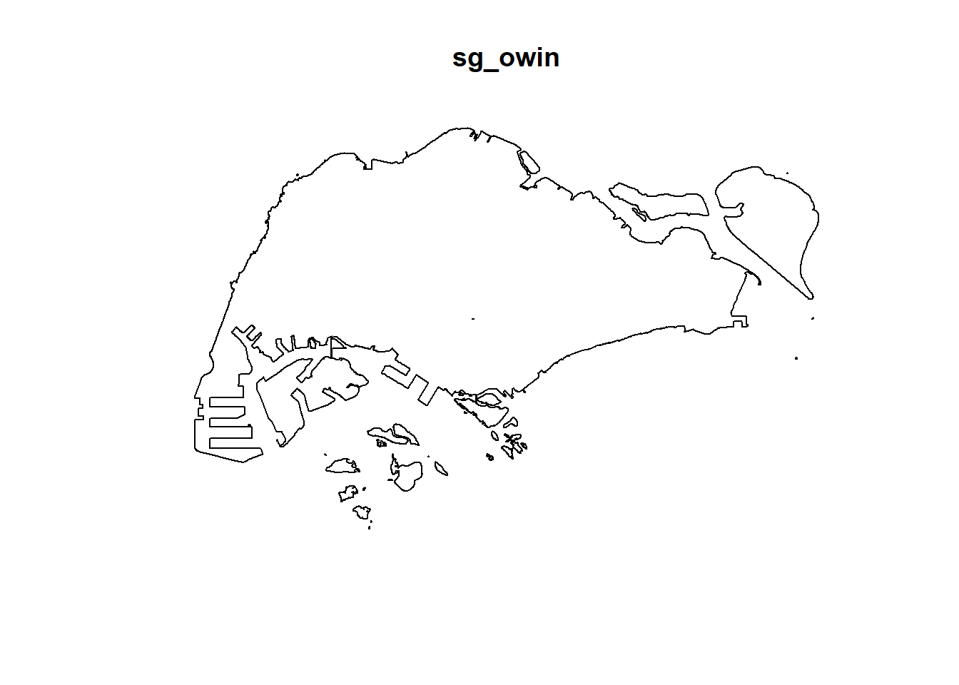
summary(sg_owin)Window: polygonal boundary
80 separate polygons (35 holes)
vertices area relative.area
polygon 1 14650 6.97996e+08 8.93e-01
polygon 2 (hole) 3 -2.21090e+00 -2.83e-09
polygon 3 285 1.61128e+06 2.06e-03
polygon 4 (hole) 3 -2.05920e-03 -2.63e-12
polygon 5 (hole) 3 -8.83647e-03 -1.13e-11
polygon 6 668 5.40368e+07 6.91e-02
polygon 7 44 2.26577e+03 2.90e-06
polygon 8 27 1.50315e+04 1.92e-05
polygon 9 711 1.28815e+07 1.65e-02
polygon 10 (hole) 36 -4.01660e+04 -5.14e-05
polygon 11 (hole) 317 -5.11280e+04 -6.54e-05
polygon 12 (hole) 3 -3.41405e-01 -4.37e-10
polygon 13 (hole) 3 -2.89050e-05 -3.70e-14
polygon 14 77 3.29939e+05 4.22e-04
polygon 15 30 2.80002e+04 3.58e-05
polygon 16 (hole) 3 -2.83151e-01 -3.62e-10
polygon 17 71 8.18750e+03 1.05e-05
polygon 18 (hole) 3 -1.68316e-04 -2.15e-13
polygon 19 (hole) 36 -7.79904e+03 -9.97e-06
polygon 20 (hole) 4 -2.05611e-02 -2.63e-11
polygon 21 (hole) 3 -2.18000e-06 -2.79e-15
polygon 22 (hole) 3 -3.65501e-03 -4.67e-12
polygon 23 (hole) 3 -4.95057e-02 -6.33e-11
polygon 24 (hole) 3 -3.99521e-02 -5.11e-11
polygon 25 (hole) 3 -6.62377e-01 -8.47e-10
polygon 26 (hole) 3 -2.09065e-03 -2.67e-12
polygon 27 91 1.49663e+04 1.91e-05
polygon 28 (hole) 26 -1.25665e+03 -1.61e-06
polygon 29 (hole) 349 -1.21433e+03 -1.55e-06
polygon 30 (hole) 20 -4.39069e+00 -5.62e-09
polygon 31 (hole) 48 -1.38338e+02 -1.77e-07
polygon 32 (hole) 28 -1.99862e+01 -2.56e-08
polygon 33 40 1.38607e+04 1.77e-05
polygon 34 (hole) 40 -6.00381e+03 -7.68e-06
polygon 35 (hole) 7 -1.40545e-01 -1.80e-10
polygon 36 (hole) 12 -8.36709e+01 -1.07e-07
polygon 37 45 2.51218e+03 3.21e-06
polygon 38 142 3.22293e+03 4.12e-06
polygon 39 148 3.10395e+03 3.97e-06
polygon 40 75 1.73526e+04 2.22e-05
polygon 41 83 5.28920e+03 6.76e-06
polygon 42 211 4.70521e+05 6.02e-04
polygon 43 106 3.04104e+03 3.89e-06
polygon 44 266 1.50631e+06 1.93e-03
polygon 45 71 5.63061e+03 7.20e-06
polygon 46 10 1.99717e+02 2.55e-07
polygon 47 478 2.06120e+06 2.64e-03
polygon 48 155 2.67502e+05 3.42e-04
polygon 49 1027 1.27782e+06 1.63e-03
polygon 50 (hole) 3 -1.16959e-03 -1.50e-12
polygon 51 65 8.42861e+04 1.08e-04
polygon 52 47 3.82087e+04 4.89e-05
polygon 53 6 4.50259e+02 5.76e-07
polygon 54 132 9.53357e+04 1.22e-04
polygon 55 (hole) 3 -3.23310e-04 -4.13e-13
polygon 56 4 2.69313e+02 3.44e-07
polygon 57 (hole) 3 -1.46474e-03 -1.87e-12
polygon 58 1045 4.44510e+06 5.68e-03
polygon 59 22 6.74651e+03 8.63e-06
polygon 60 64 3.43149e+04 4.39e-05
polygon 61 (hole) 3 -1.98390e-03 -2.54e-12
polygon 62 (hole) 4 -1.13774e-02 -1.46e-11
polygon 63 14 5.86546e+03 7.50e-06
polygon 64 95 5.96187e+04 7.62e-05
polygon 65 (hole) 4 -1.86410e-02 -2.38e-11
polygon 66 (hole) 3 -5.12482e-03 -6.55e-12
polygon 67 (hole) 3 -1.96410e-03 -2.51e-12
polygon 68 (hole) 3 -5.55856e-03 -7.11e-12
polygon 69 234 2.08755e+06 2.67e-03
polygon 70 10 4.90942e+02 6.28e-07
polygon 71 234 4.72886e+05 6.05e-04
polygon 72 (hole) 13 -3.91907e+02 -5.01e-07
polygon 73 15 4.03300e+04 5.16e-05
polygon 74 227 1.10308e+06 1.41e-03
polygon 75 10 6.60195e+03 8.44e-06
polygon 76 19 3.09221e+04 3.95e-05
polygon 77 145 9.61782e+05 1.23e-03
polygon 78 30 4.28933e+03 5.49e-06
polygon 79 37 1.29481e+04 1.66e-05
polygon 80 4 9.47108e+01 1.21e-07
enclosing rectangle: [2667.54, 56396.44] x [15748.72, 50256.33] units
(53730 x 34510 units)
Window area = 781945000 square units
Fraction of frame area: 0.4222.9 Combining the point events object and owin object
childcareSG_ppp = childcare_ppp[sg_owin]Following which the output combines both the point and polygon feature in one ppp object class as shown in the code chunk below.
plot(childcareSG_ppp)Warning in default.charmap(ntypes, chars): Too many types to display every type
as a different characterWarning: Only 10 out of 1545 symbols are shown in the symbol map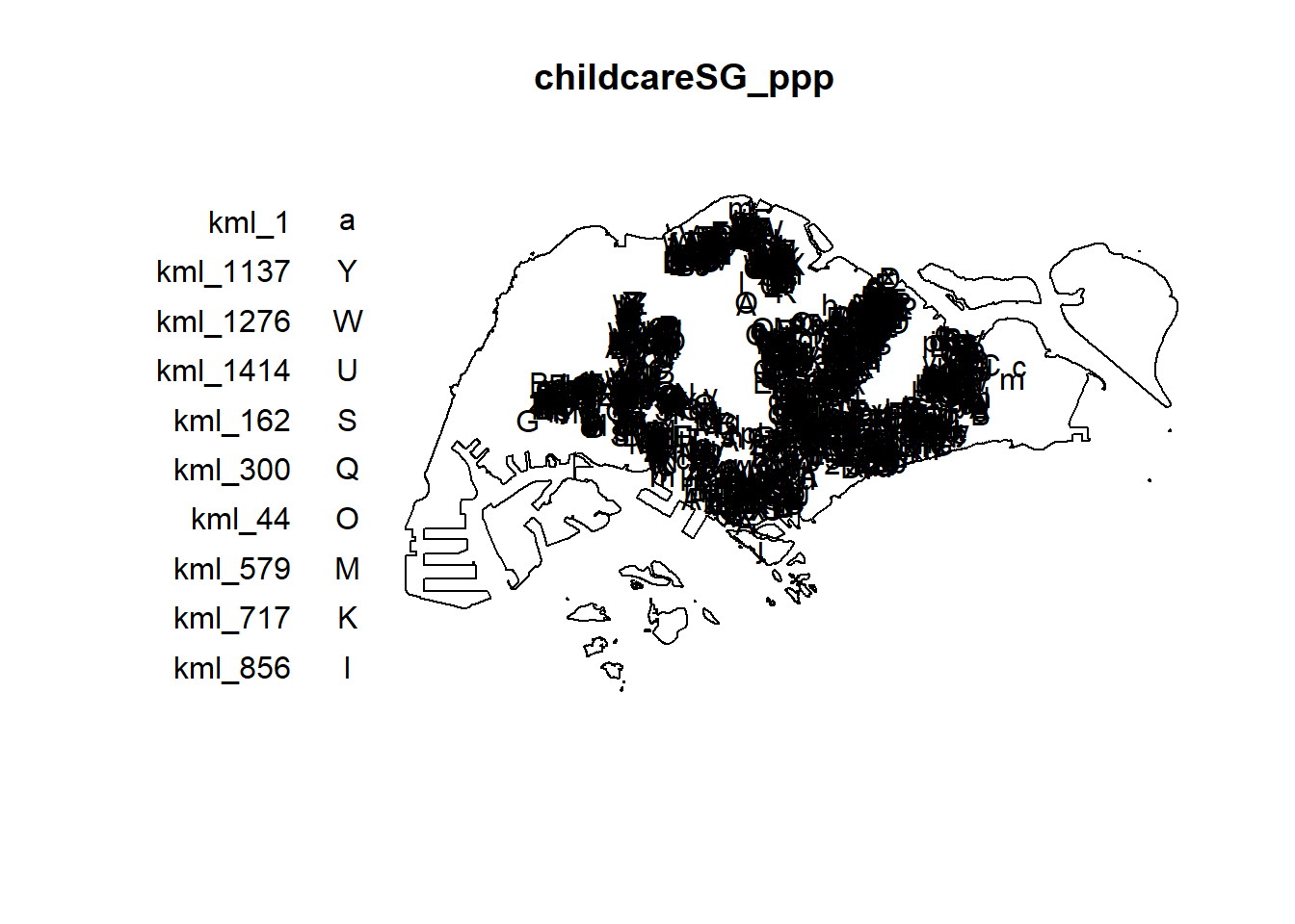
2.10 Kernel Density Estimation of Spatial Point Events
Code chunk below is used to re-scale the unit of measurement from metres to kilometres before KDE is performed.
childcareSG_ppp.km <- rescale.ppp(childcareSG_ppp, 1000, "km")kde_childcareSG_adaptive <- adaptive.density(childcareSG_ppp.km,
method = "kernel")
plot(kde_childcareSG_adaptive)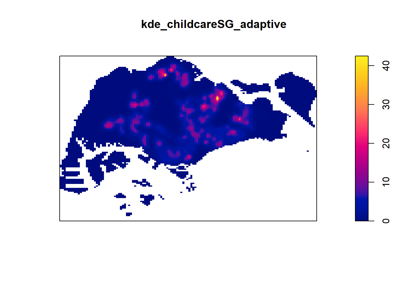
2.11 Kernel Density Estimation
The code chunk shows two different ways to convert KDE output into grid objects
maptool must be installed for this method
par(bg = '#E4D5C9')gridded_kde_childcareSG_ad <- maptools::as.SpatialGridDataFrame.im(
kde_childcareSG_adaptive)Please note that 'maptools' will be retired during October 2023,
plan transition at your earliest convenience (see
https://r-spatial.org/r/2023/05/15/evolution4.html and earlier blogs
for guidance);some functionality will be moved to 'sp'.
Checking rgeos availability: FALSEspplot(gridded_kde_childcareSG_ad)
gridded_kde_childcareSG_ad <- as(kde_childcareSG_adaptive,
                                 "SpatialGridDataFrame")

spplot(gridded_kde_childcareSG_ad)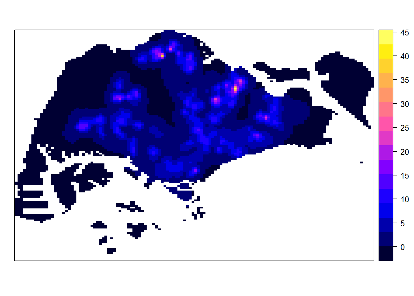
Both methods have simialr or otherwise the same results however usage if spatstat.geom is preferred as maptools has been retired
2.12 Monte Carlo Simulation
Tip
In order to ensure reproducibility, it is important to include the code chunk below before using spatial spatstat functions involving Monte Carlo simulation
Without doing so f values for instance might change each time the code chunk is ran.
set.seed(1234)2.14 The datasets
For this case study, three basic data sets are needed, they are:
2.15 Importing the Traffic Accident Data
Importing the downloaded accident data into R environment and saving the output as an sf tibble data.frame.
rdacc_sf <- read_csv("data/Thailand/archive/thai_road_accident_2019_2022.csv") %>%
  filter(!is.na(longitude) & longitude != "",
         !is.na(latitude) & latitude != "") %>%
  st_as_sf(coords = c(
    "longitude", "latitude"),
    crs = 4326) %>%
  st_transform(crs = 32647)
Rows: 81735 Columns: 18
── Column specification ────────────────────────────────────────────────────────
Delimiter: ","
chr (10): province_th, province_en, agency, route, vehicle_type, presumed_c...
dbl (6): acc_code, number_of_vehicles_involved, number_of_fatalities, numb...
dttm (2): incident_datetime, report_datetime
ℹ Use `spec()` to retrieve the full column specification for this data.
ℹ Specify the column types or set `show_col_types = FALSE` to quiet this message.2.16 Visualising The Accident Data
Importing the ACLED data into R environment as an sf tibble data.frame.